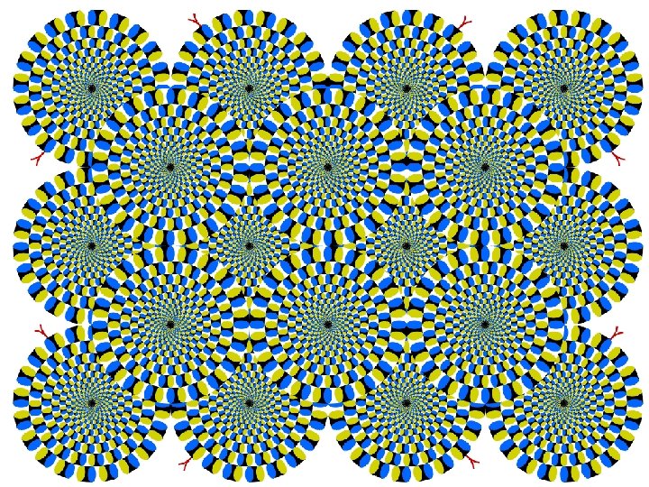
Motion illusion rotating snakes Does it work on







- Slides: 68


Motion illusion, rotating snakes

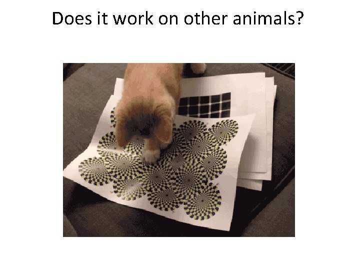
Does it work on other animals?

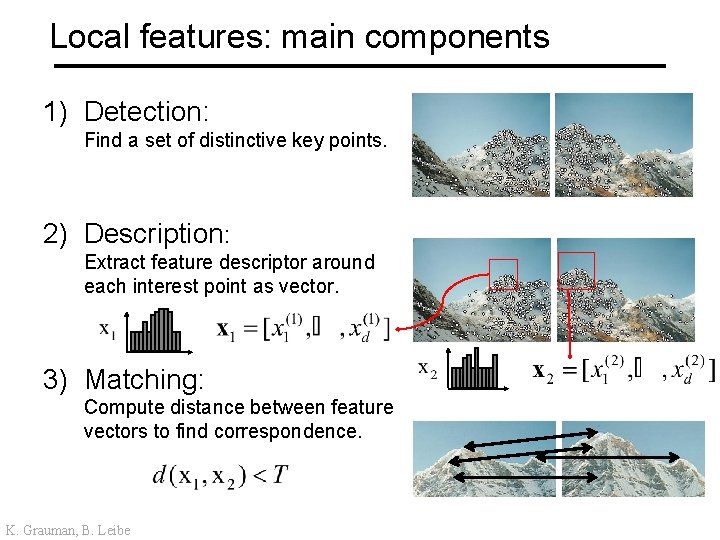
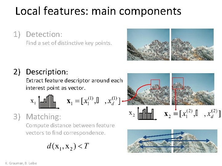
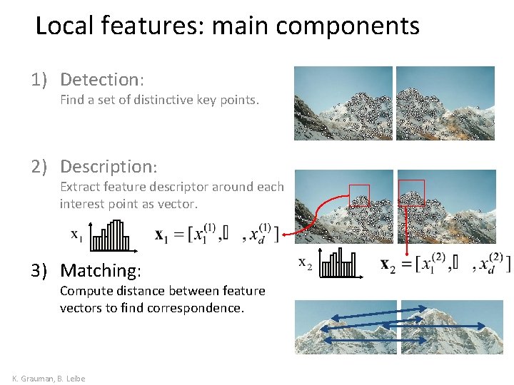
Local features: main components 1) Detection: Find a set of distinctive key points. 2) Description: Extract feature descriptor around each interest point as vector. 3) Matching: Compute distance between feature vectors to find correspondence. K. Grauman, B. Leibe

HOW INVARIANT ARE HARRIS CORNERS?

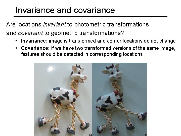
Invariance and covariance Are locations invariant to photometric transformations and covariant to geometric transformations? • Invariance: image is transformed and corner locations do not change • Covariance: if we have two transformed versions of the same image, features should be detected in corresponding locations

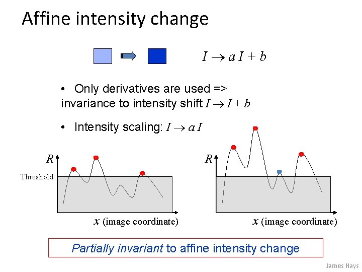
Affine intensity change I a. I+b • Only derivatives are used => invariance to intensity shift I I + b • Intensity scaling: I a I R R Threshold x (image coordinate) Partially invariant to affine intensity change James Hays


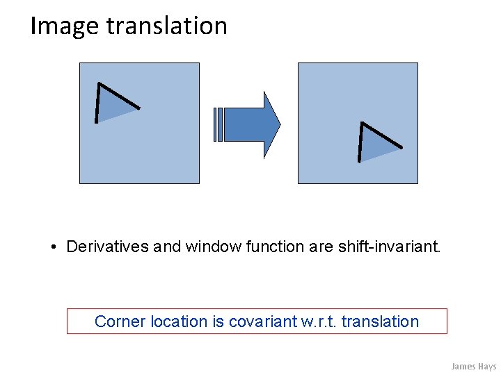
Image translation • Derivatives and window function are shift-invariant. Corner location is covariant w. r. t. translation James Hays

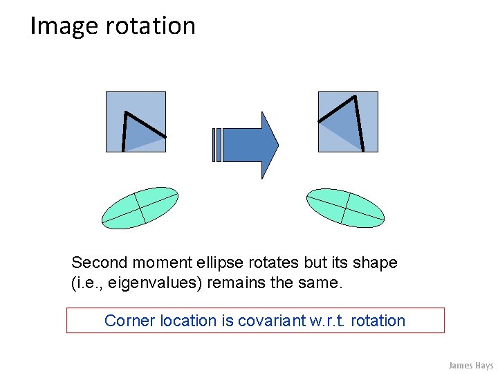
Image rotation Second moment ellipse rotates but its shape (i. e. , eigenvalues) remains the same. Corner location is covariant w. r. t. rotation James Hays

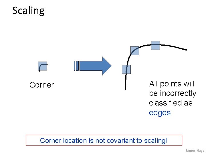
Scaling Corner All points will be incorrectly classified as edges Corner location is not covariant to scaling! James Hays

WHAT IS THE ‘SCALE’ OF A FEATURE POINT?

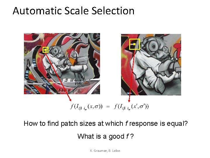
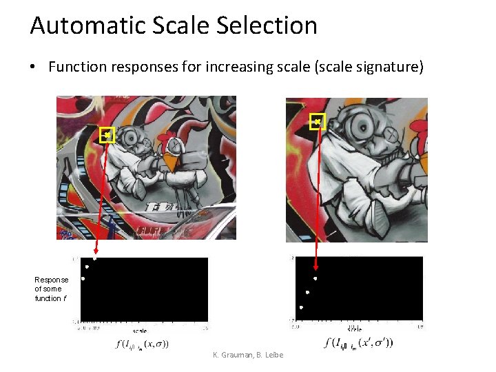
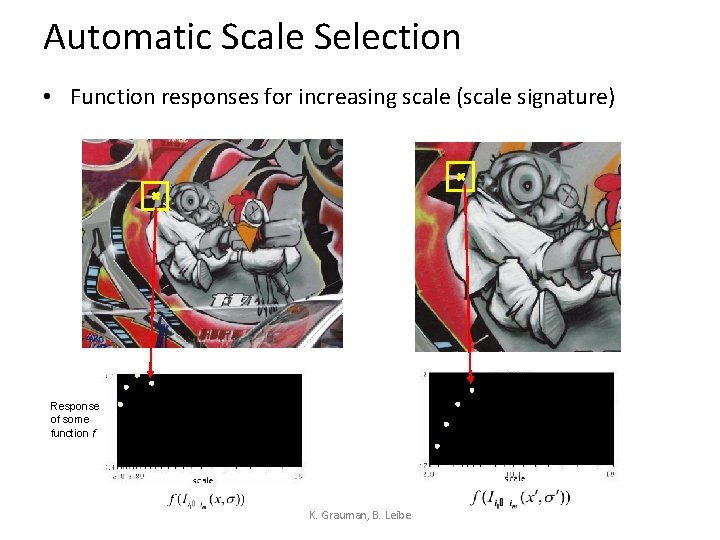
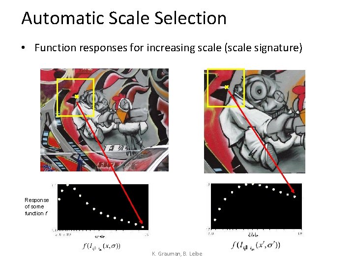
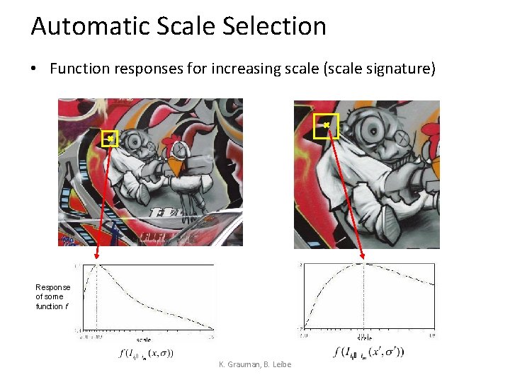
Automatic Scale Selection How to find patch sizes at which f response is equal? What is a good f ? K. Grauman, B. Leibe

Automatic Scale Selection • Function responses for increasing scale (scale signature) Response of some function f K. Grauman, B. Leibe

Automatic Scale Selection • Function responses for increasing scale (scale signature) Response of some function f K. Grauman, B. Leibe

Automatic Scale Selection • Function responses for increasing scale (scale signature) Response of some function f K. Grauman, B. Leibe

Automatic Scale Selection • Function responses for increasing scale (scale signature) Response of some function f K. Grauman, B. Leibe

Automatic Scale Selection • Function responses for increasing scale (scale signature) Response of some function f K. Grauman, B. Leibe

Automatic Scale Selection • Function responses for increasing scale (scale signature) Response of some function f K. Grauman, B. Leibe

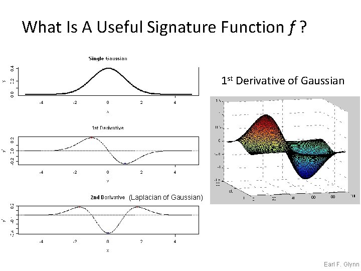
What Is A Useful Signature Function f ? 1 st Derivative of Gaussian (Laplacian of Gaussian) Earl F. Glynn

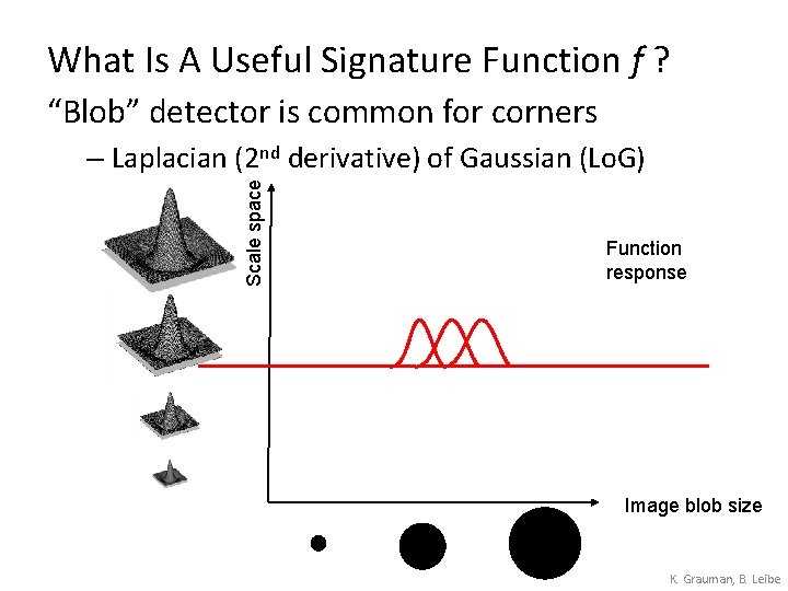
What Is A Useful Signature Function f ? “Blob” detector is common for corners Scale space – Laplacian (2 nd derivative) of Gaussian (Lo. G) Function response Image blob size K. Grauman, B. Leibe

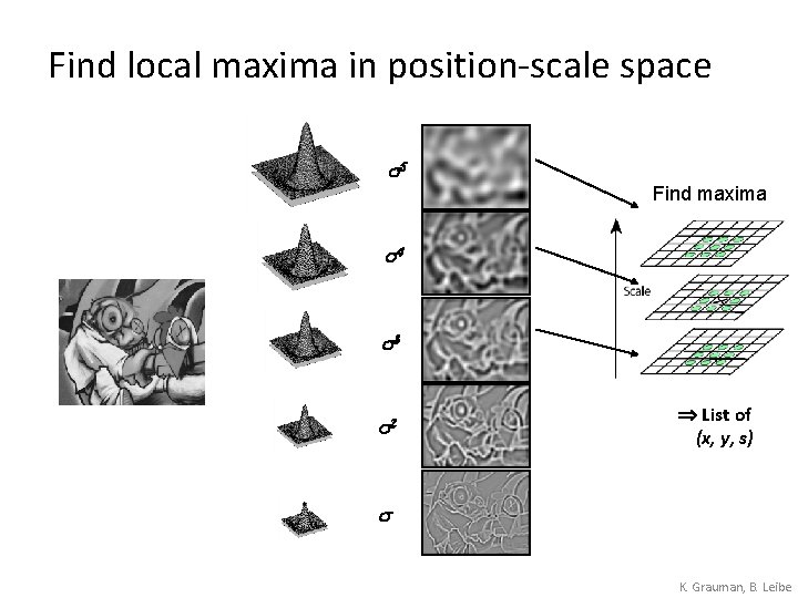
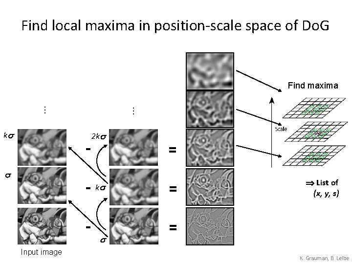
Find local maxima in position-scale space s 5 Find maxima s 4 s 3 s 2 List of (x, y, s) s K. Grauman, B. Leibe

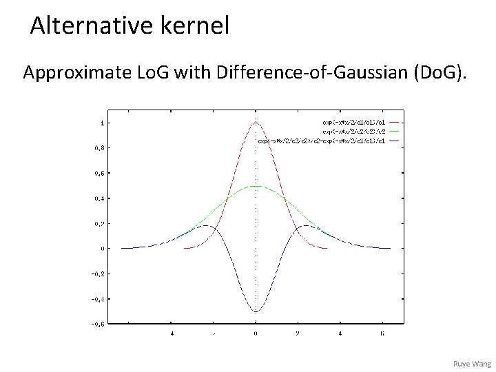
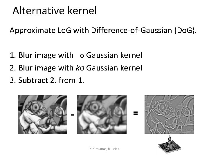
Alternative kernel Approximate Lo. G with Difference-of-Gaussian (Do. G). Ruye Wang

Alternative kernel Approximate Lo. G with Difference-of-Gaussian (Do. G). 1. Blur image with σ Gaussian kernel 2. Blur image with kσ Gaussian kernel 3. Subtract 2. from 1. = - K. Grauman, B. Leibe

Find local maxima in position-scale space of Do. G ks … … Find maxima - s Input image 2 ks = ks s = List of (x, y, s) = K. Grauman, B. Leibe

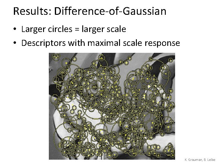
Results: Difference-of-Gaussian • Larger circles = larger scale • Descriptors with maximal scale response K. Grauman, B. Leibe

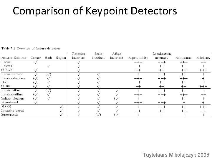
Comparison of Keypoint Detectors Tuytelaars Mikolajczyk 2008

Local Image Descriptors Read Szeliski 4. 1 Acknowledgment: Many slides from James Hays, Derek Hoiem and Grauman & Leibe 2008 AAAI Tutorial

Local features: main components 1) Detection: Find a set of distinctive key points. 2) Description: Extract feature descriptor around each interest point as vector. 3) Matching: Compute distance between feature vectors to find correspondence. K. Grauman, B. Leibe

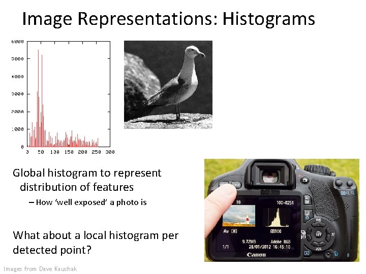
Image Representations: Histograms Global histogram to represent distribution of features – How ‘well exposed’ a photo is What about a local histogram per detected point? Images from Dave Kauchak Space Shuttle Cargo Bay

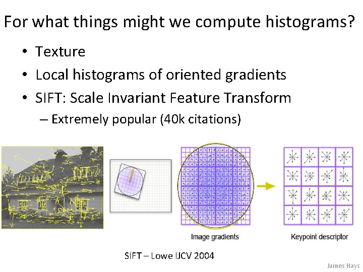
For what things might we compute histograms? • Texture • Local histograms of oriented gradients • SIFT: Scale Invariant Feature Transform – Extremely popular (40 k citations) SIFT – Lowe IJCV 2004 James Hays

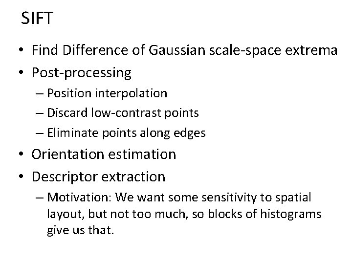
SIFT preprocessing • Find Difference of Gaussian scale-space extrema as feature point locations • Post-processing – Subpixel position interpolation – Discard low-contrast points – Eliminate points along edges • Orientation estimation per feature point

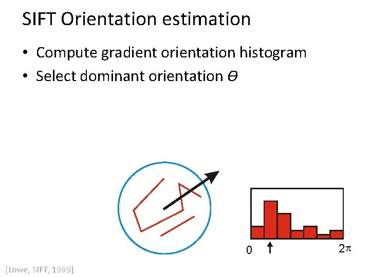
SIFT Orientation estimation • Compute gradient orientation histogram • Select dominant orientation ϴ 0 [Lowe, SIFT, 1999] T. Tuytelaars, B. Leibe 2 p

SIFT • Find Difference of Gaussian scale-space extrema • Post-processing – Position interpolation – Discard low-contrast points – Eliminate points along edges • Orientation estimation • Descriptor extraction – Motivation: We want some sensitivity to spatial layout, but not too much, so blocks of histograms give us that.

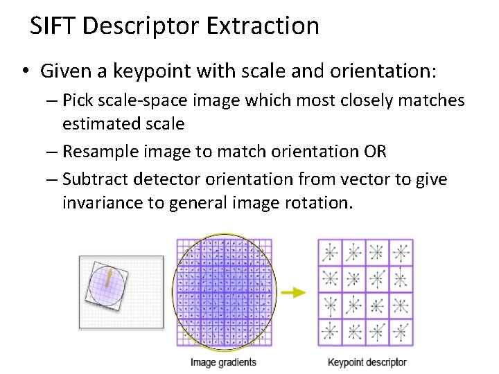
SIFT Descriptor Extraction • Given a keypoint with scale and orientation: – Pick scale-space image which most closely matches estimated scale – Resample image to match orientation OR – Subtract detector orientation from vector to give invariance to general image rotation.

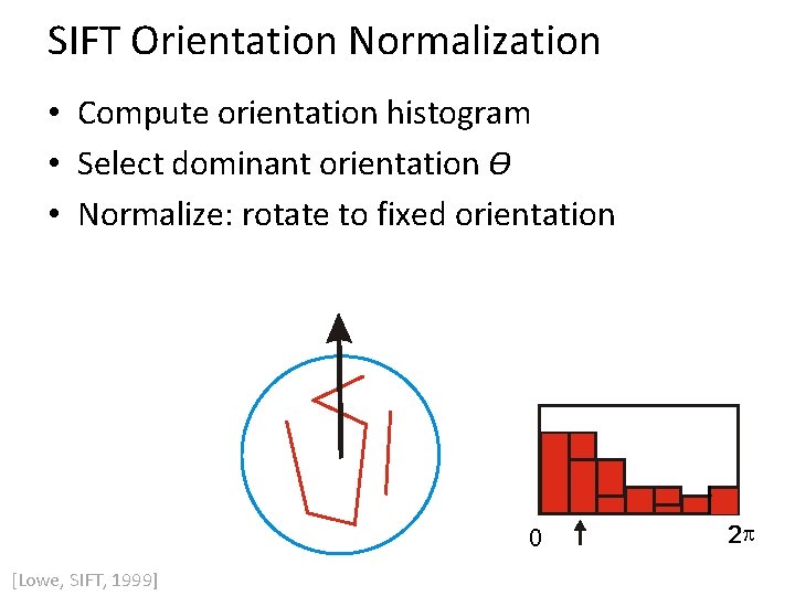
SIFT Orientation Normalization • Compute orientation histogram • Select dominant orientation ϴ • Normalize: rotate to fixed orientation 0 [Lowe, SIFT, 1999] T. Tuytelaars, B. Leibe 2 p

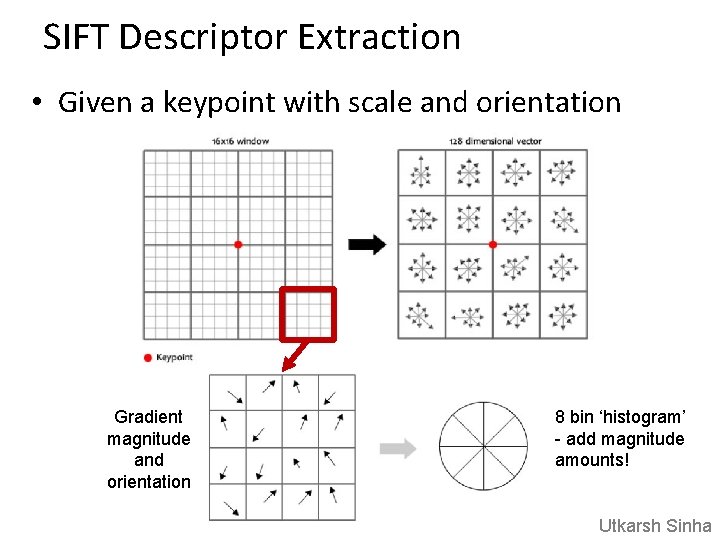
SIFT Descriptor Extraction • Given a keypoint with scale and orientation Gradient magnitude and orientation 8 bin ‘histogram’ - add magnitude amounts! Utkarsh Sinha

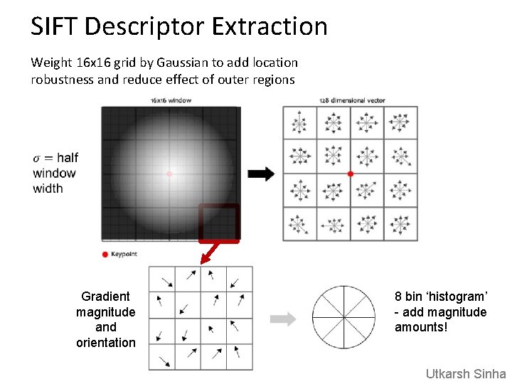
SIFT Descriptor Extraction Weight 16 x 16 grid by Gaussian to add location robustness and reduce effect of outer regions Gradient magnitude and orientation 8 bin ‘histogram’ - add magnitude amounts! Utkarsh Sinha

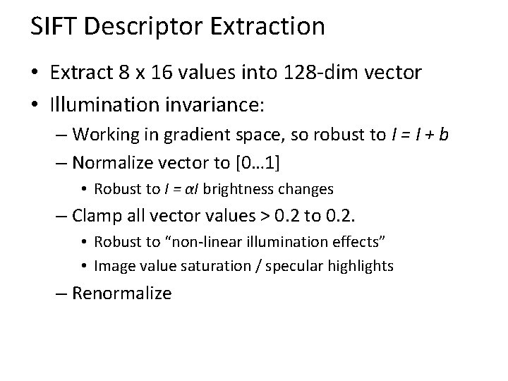
SIFT Descriptor Extraction • Extract 8 x 16 values into 128 -dim vector • Illumination invariance: – Working in gradient space, so robust to I = I + b – Normalize vector to [0… 1] • Robust to I = αI brightness changes – Clamp all vector values > 0. 2 to 0. 2. • Robust to “non-linear illumination effects” • Image value saturation / specular highlights – Renormalize

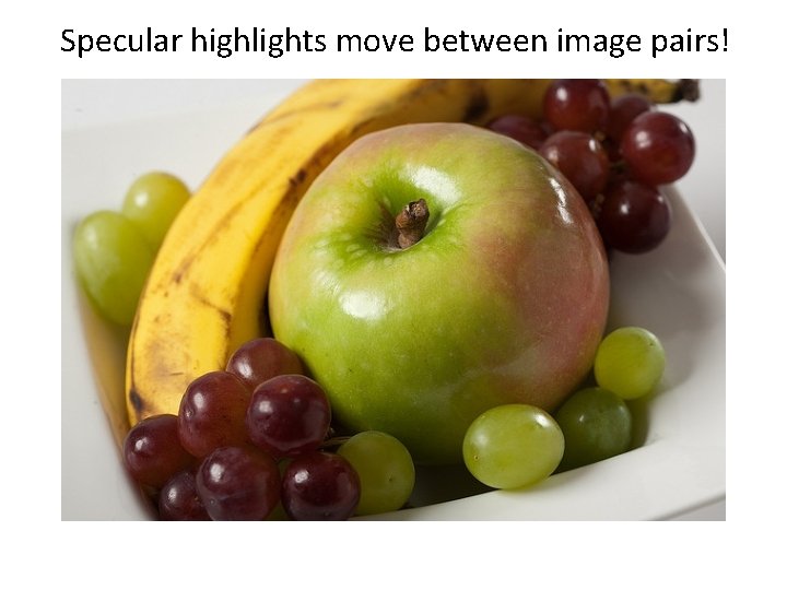
Specular highlights move between image pairs!

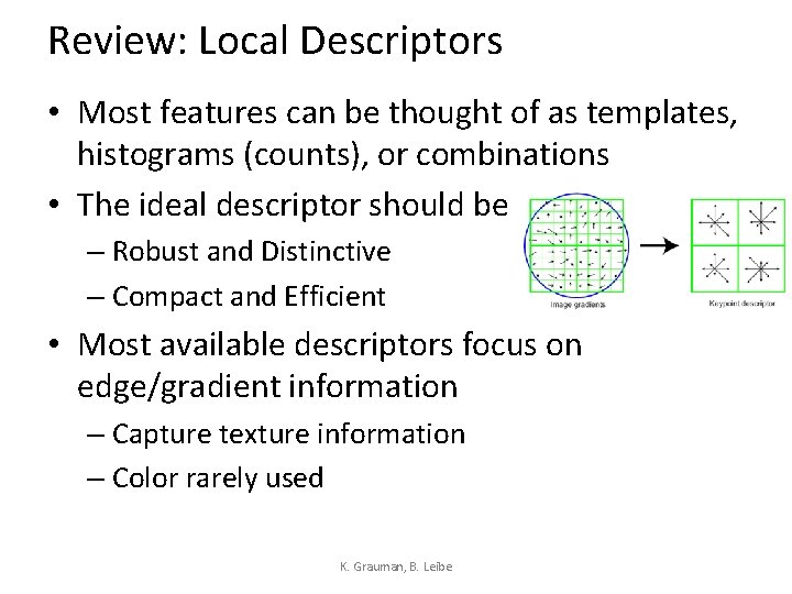
Review: Local Descriptors • Most features can be thought of as templates, histograms (counts), or combinations • The ideal descriptor should be – Robust and Distinctive – Compact and Efficient • Most available descriptors focus on edge/gradient information – Capture texture information – Color rarely used K. Grauman, B. Leibe


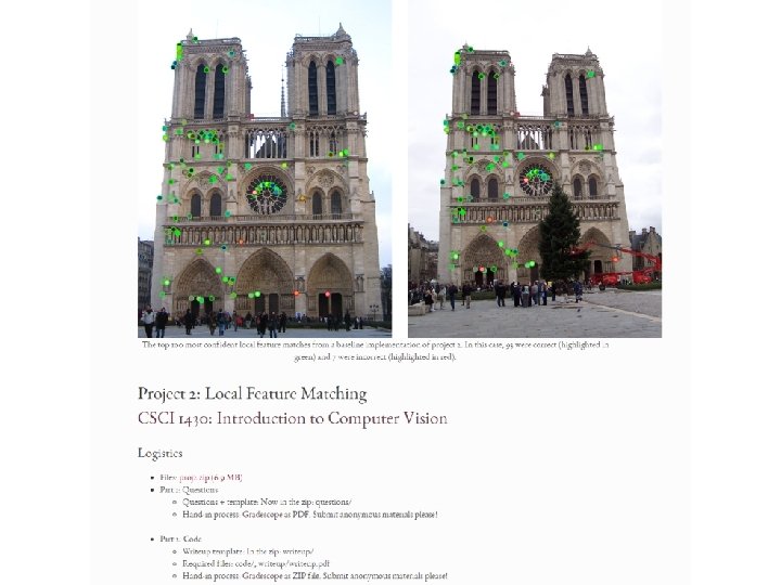
SIFT-like descriptor in Project 2 • SIFT is hand designed based on intuition • You implement your own SIFT-like descriptor – Ignore scale/orientation to start. • Parameters: stick with defaults + minor tweaks • Feel free to look at papers / resources for inspiration Lowe’s original paper: http: //www. cs. ubc. ca/~lowe/papers/ijcv 04. pdf 70

Feature Matching Read Szeliski 4. 1 Many slides from James Hays, Derek Hoiem, and Grauman&Leibe 2008 AAAI Tutorial

Local features: main components 1) Detection: Find a set of distinctive key points. 2) Description: Extract feature descriptor around each interest point as vector. 3) Matching: Compute distance between feature vectors to find correspondence. K. Grauman, B. Leibe

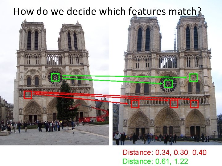
How do we decide which features match? Distance: 0. 34, 0. 30, 0. 40 Distance: 0. 61, 1. 22

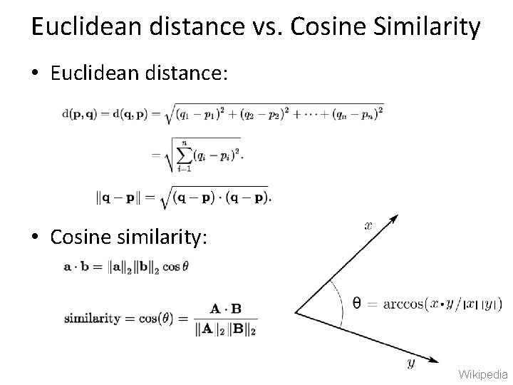
Euclidean distance vs. Cosine Similarity • Euclidean distance: • Cosine similarity: Wikipedia

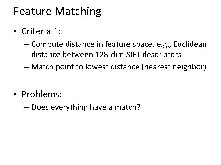
Feature Matching • Criteria 1: – Compute distance in feature space, e. g. , Euclidean distance between 128 -dim SIFT descriptors – Match point to lowest distance (nearest neighbor) • Problems: – Does everything have a match?

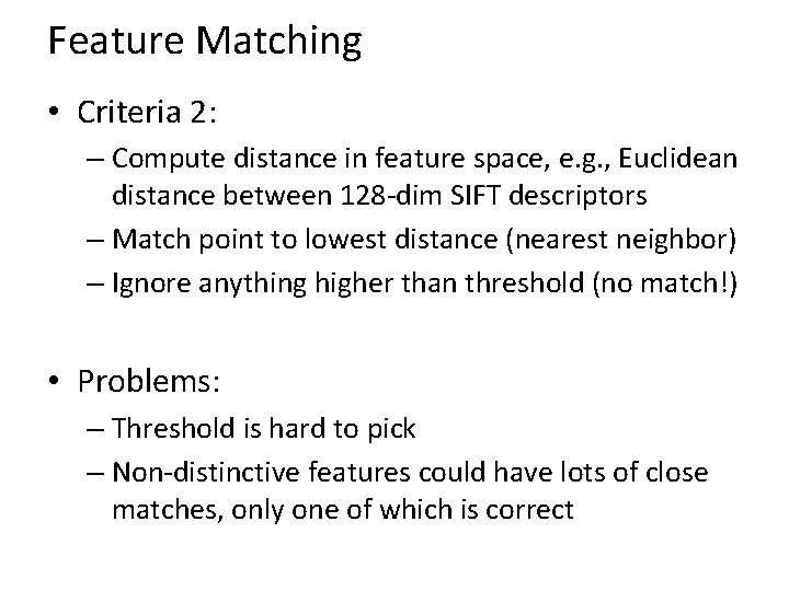
Feature Matching • Criteria 2: – Compute distance in feature space, e. g. , Euclidean distance between 128 -dim SIFT descriptors – Match point to lowest distance (nearest neighbor) – Ignore anything higher than threshold (no match!) • Problems: – Threshold is hard to pick – Non-distinctive features could have lots of close matches, only one of which is correct

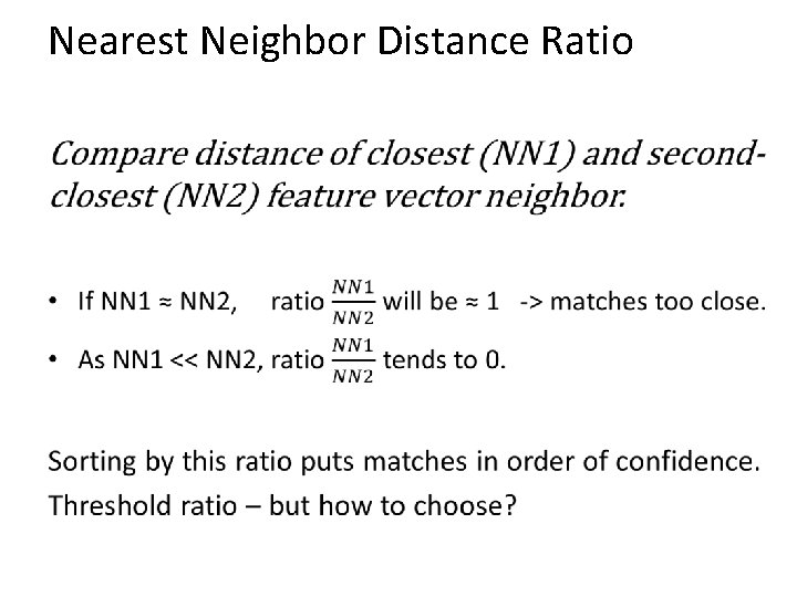
Nearest Neighbor Distance Ratio •

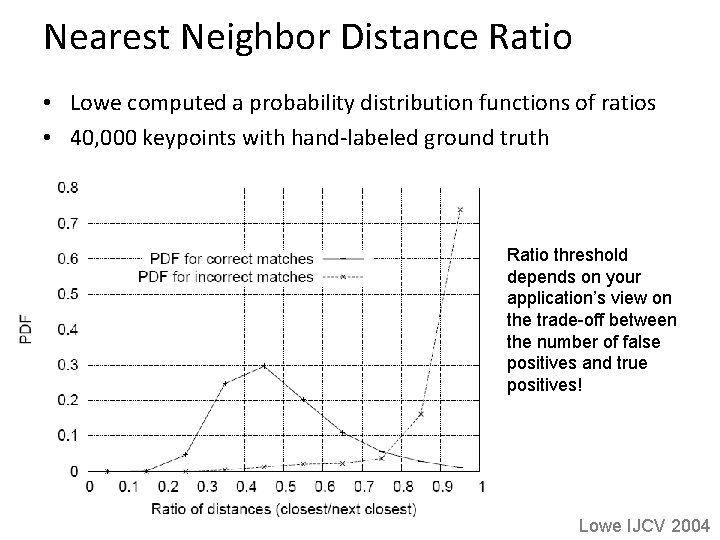
Nearest Neighbor Distance Ratio • Lowe computed a probability distribution functions of ratios • 40, 000 keypoints with hand-labeled ground truth Ratio threshold depends on your application’s view on the trade-off between the number of false positives and true positives! Lowe IJCV 2004

Efficient compute cost • Naïve looping: Expensive • Operate on matrices of descriptors • E. g. , for row vectors, features_image 1 * features_image 2 T produces matrix of dot product results for all pairs of features

Live SIFT Demo Actually a similar alternative, called SURF. Speeded-Up Robust Features Bay et al. , ECCV 2006 (Both are patented; SURF has noncommercial license. )

HOW GOOD IS SIFT?

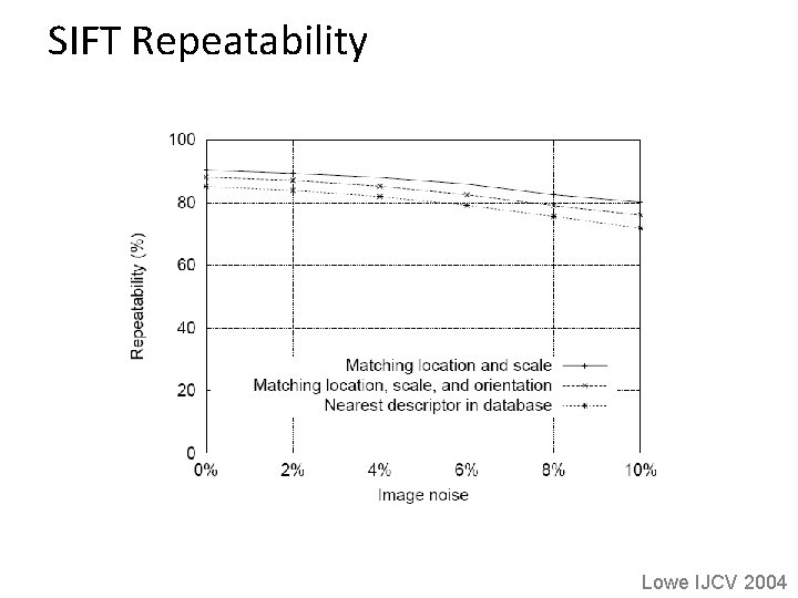
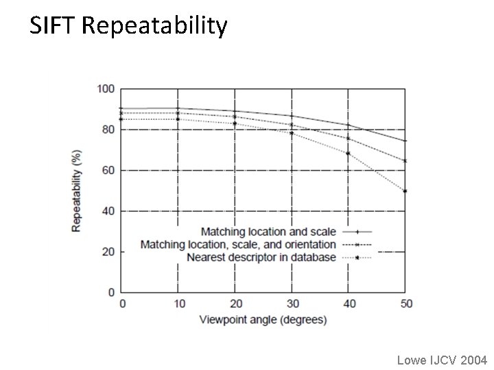
SIFT Repeatability Lowe IJCV 2004

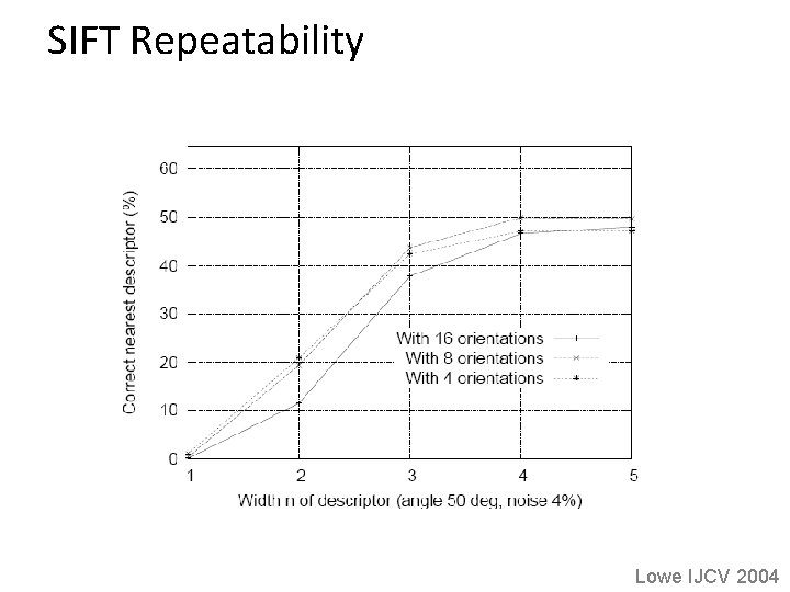
SIFT Repeatability Lowe IJCV 2004

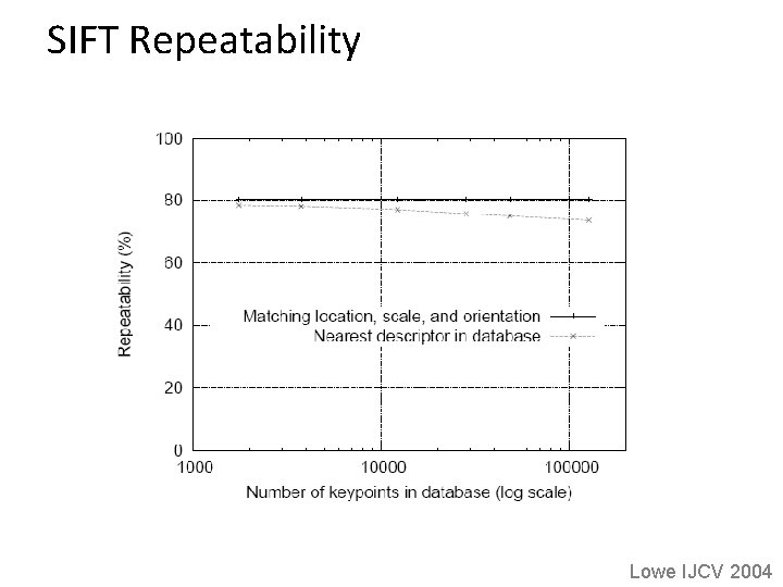
SIFT Repeatability Lowe IJCV 2004

SIFT Repeatability Lowe IJCV 2004

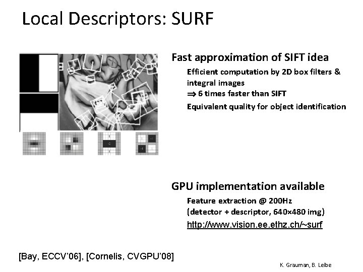
Local Descriptors: SURF • Fast approximation of SIFT idea Ø Ø Efficient computation by 2 D box filters & integral images 6 times faster than SIFT Equivalent quality for object identification • GPU implementation available Ø Ø [Bay, ECCV’ 06], [Cornelis, CVGPU’ 08] Feature extraction @ 200 Hz (detector + descriptor, 640× 480 img) http: //www. vision. ee. ethz. ch/~surf K. Grauman, B. Leibe

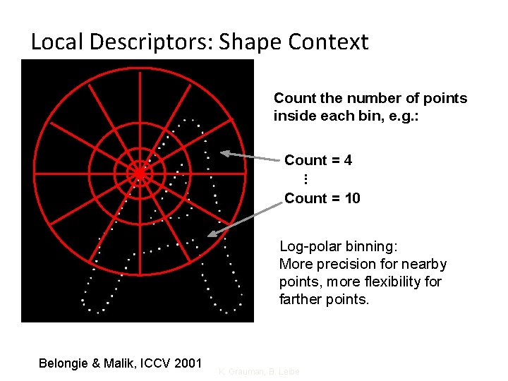
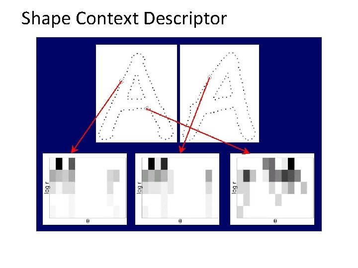
Local Descriptors: Shape Context Count the number of points inside each bin, e. g. : Count = 4. . . Count = 10 Log-polar binning: More precision for nearby points, more flexibility for farther points. Belongie & Malik, ICCV 2001 K. Grauman, B. Leibe

Shape Context Descriptor

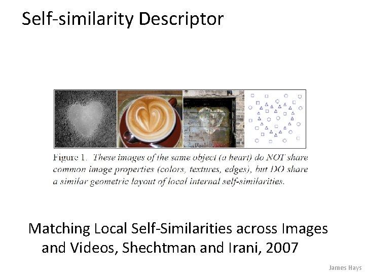
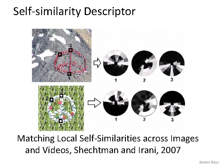
Self-similarity Descriptor Matching Local Self-Similarities across Images and Videos, Shechtman and Irani, 2007 James Hays

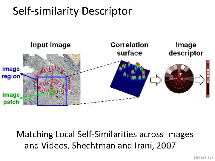
Self-similarity Descriptor Matching Local Self-Similarities across Images and Videos, Shechtman and Irani, 2007 James Hays

Self-similarity Descriptor Matching Local Self-Similarities across Images and Videos, Shechtman and Irani, 2007 James Hays

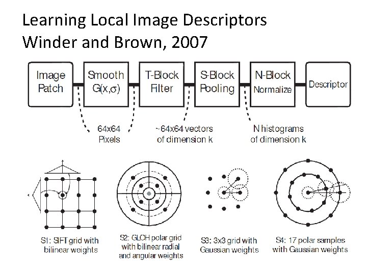
Learning Local Image Descriptors Winder and Brown, 2007

Right features are application specific • Shape: scene-scale, object-scale, detail-scale – 2 D form, shading, shadows, texture, linear perspective • Material properties: albedo, feel, hardness, … – Color, texture • Motion – Optical flow, tracked points • Distance – Stereo, position, occlusion, scene shape – If known object: size, other objects

Available at a web site near you… • Many local feature detectors have executables available online: – http: //www. robots. ox. ac. uk/~vgg/research/affine – http: //www. cs. ubc. ca/~lowe/keypoints/ – http: //www. vision. ee. ethz. ch/~surf K. Grauman, B. Leibe

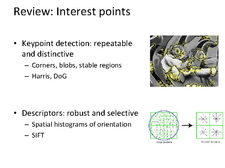
Review: Interest points • Keypoint detection: repeatable and distinctive – Corners, blobs, stable regions – Harris, Do. G • Descriptors: robust and selective – Spatial histograms of orientation – SIFT