Motion Estimation Why estimate motion Lots of uses

Motion Estimation

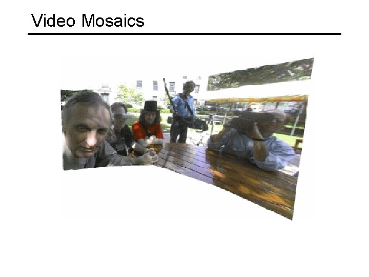
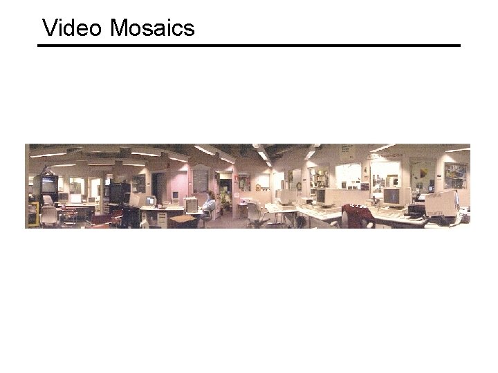
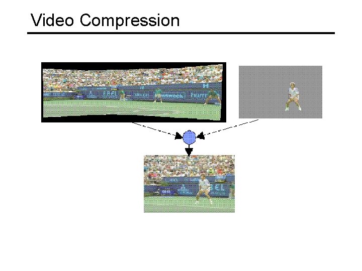
Why estimate motion? Lots of uses • • • Motion Detection Track object behavior Correct for camera jitter (stabilization) Align images (mosaics) 3 D shape reconstruction Video Compression

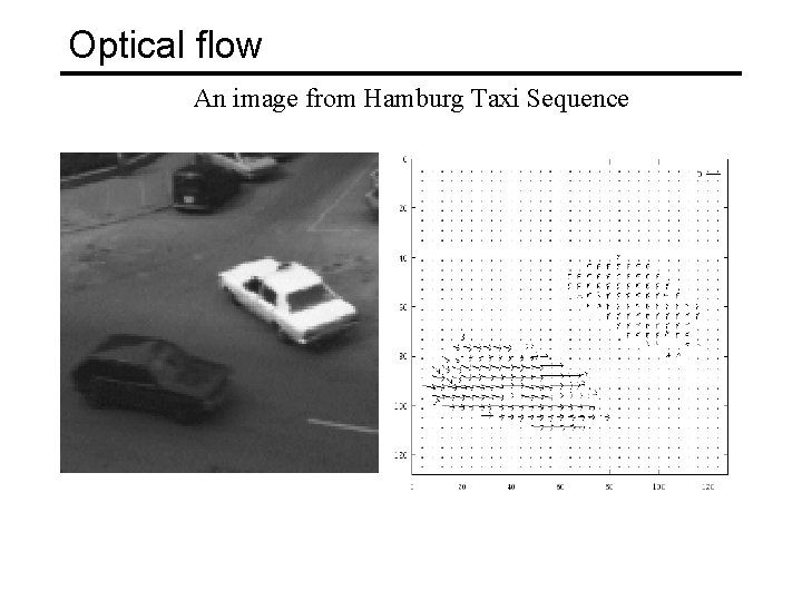
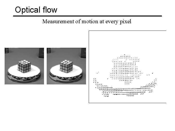
Optical flow Measurement of motion at every pixel

Optical flow An image from Hamburg Taxi Sequence

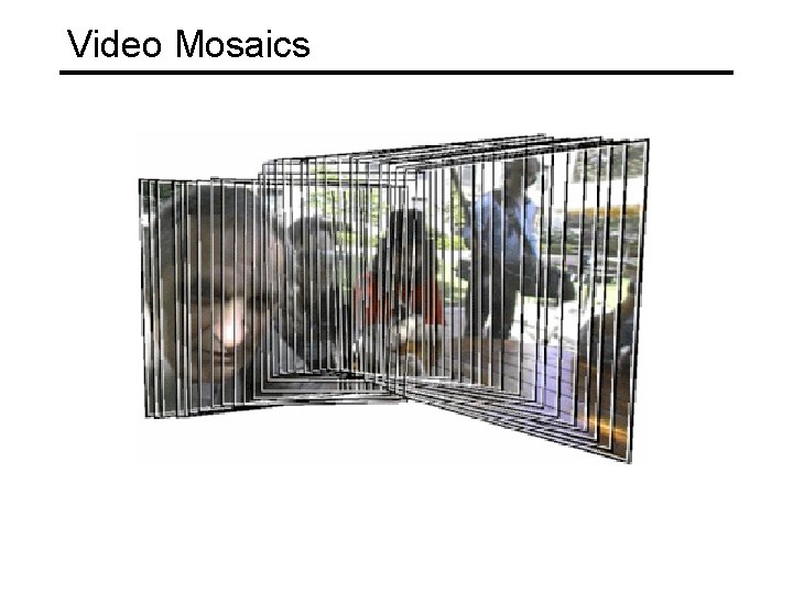
Video Mosaics

Video Mosaics

Video Mosaics

Video Compression

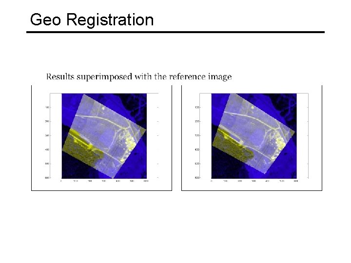
Geo Registration

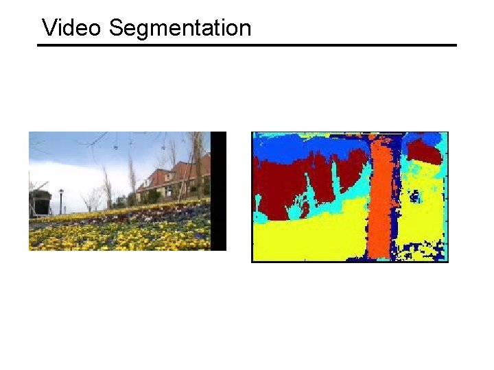
Video Segmentation

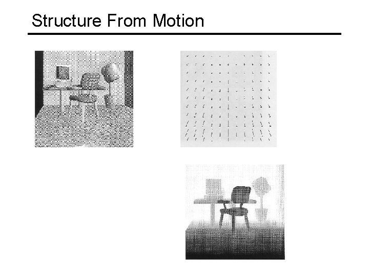
Structure From Motion

Optical flow Measurement of motion at every pixel

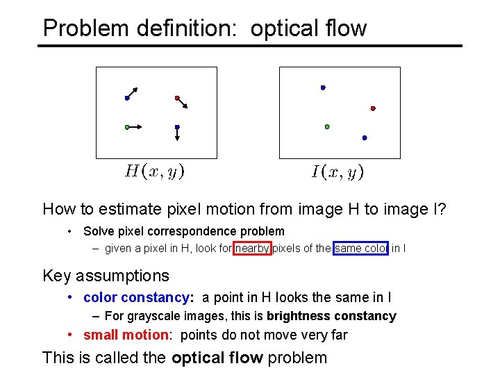
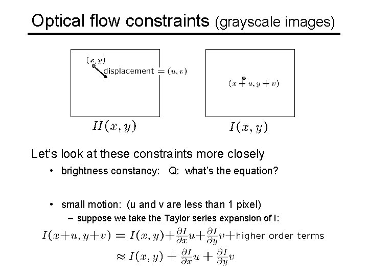
Problem definition: optical flow How to estimate pixel motion from image H to image I? • Solve pixel correspondence problem – given a pixel in H, look for nearby pixels of the same color in I Key assumptions • color constancy: a point in H looks the same in I – For grayscale images, this is brightness constancy • small motion: points do not move very far This is called the optical flow problem

Optical flow constraints (grayscale images) Let’s look at these constraints more closely • brightness constancy: Q: what’s the equation? • small motion: (u and v are less than 1 pixel) – suppose we take the Taylor series expansion of I:

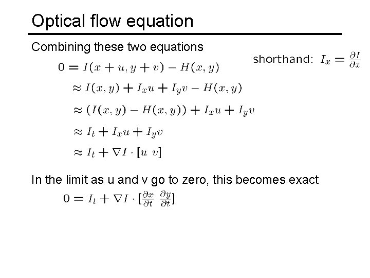
Optical flow equation Combining these two equations In the limit as u and v go to zero, this becomes exact

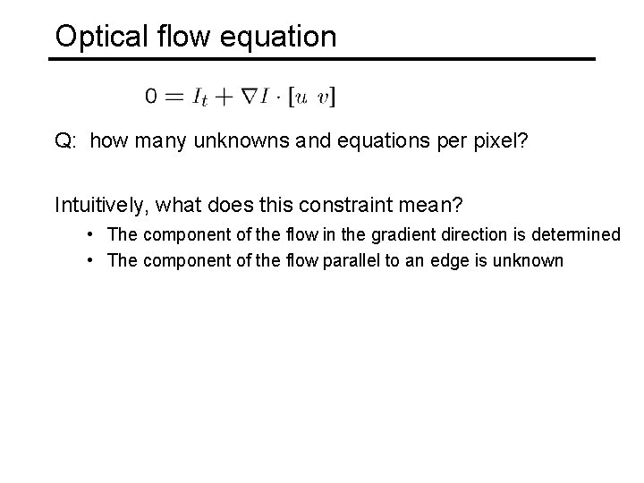
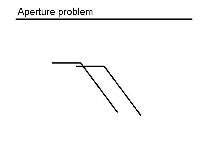
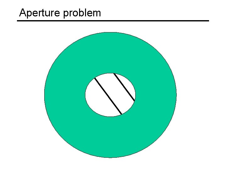
Optical flow equation Q: how many unknowns and equations per pixel? Intuitively, what does this constraint mean? • The component of the flow in the gradient direction is determined • The component of the flow parallel to an edge is unknown

Aperture problem

Aperture problem

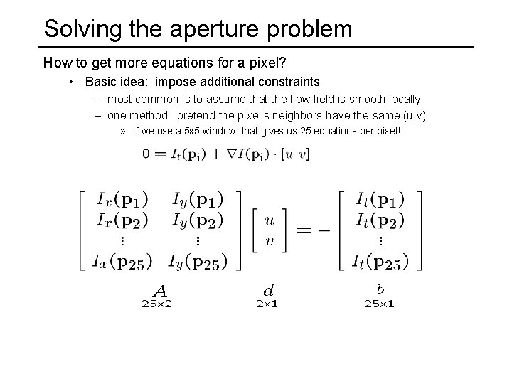
Solving the aperture problem How to get more equations for a pixel? • Basic idea: impose additional constraints – most common is to assume that the flow field is smooth locally – one method: pretend the pixel’s neighbors have the same (u, v) » If we use a 5 x 5 window, that gives us 25 equations per pixel!

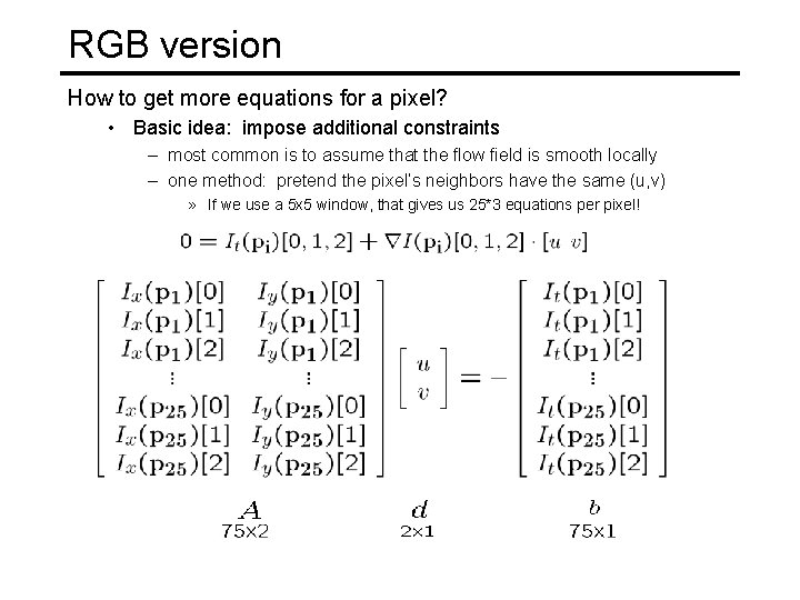
RGB version How to get more equations for a pixel? • Basic idea: impose additional constraints – most common is to assume that the flow field is smooth locally – one method: pretend the pixel’s neighbors have the same (u, v) » If we use a 5 x 5 window, that gives us 25*3 equations per pixel!

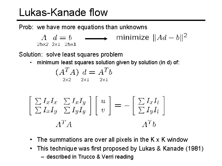
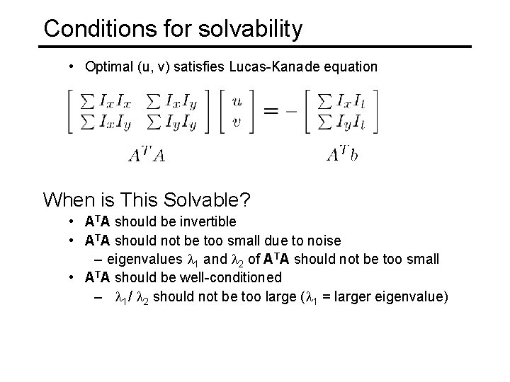
Lukas-Kanade flow Prob: we have more equations than unknowns Solution: solve least squares problem • minimum least squares solution given by solution (in d) of: • The summations are over all pixels in the K x K window • This technique was first proposed by Lukas & Kanade (1981) – described in Trucco & Verri reading

Conditions for solvability • Optimal (u, v) satisfies Lucas-Kanade equation When is This Solvable? • ATA should be invertible • ATA should not be too small due to noise – eigenvalues l 1 and l 2 of ATA should not be too small • ATA should be well-conditioned – l 1/ l 2 should not be too large (l 1 = larger eigenvalue)

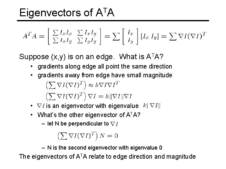
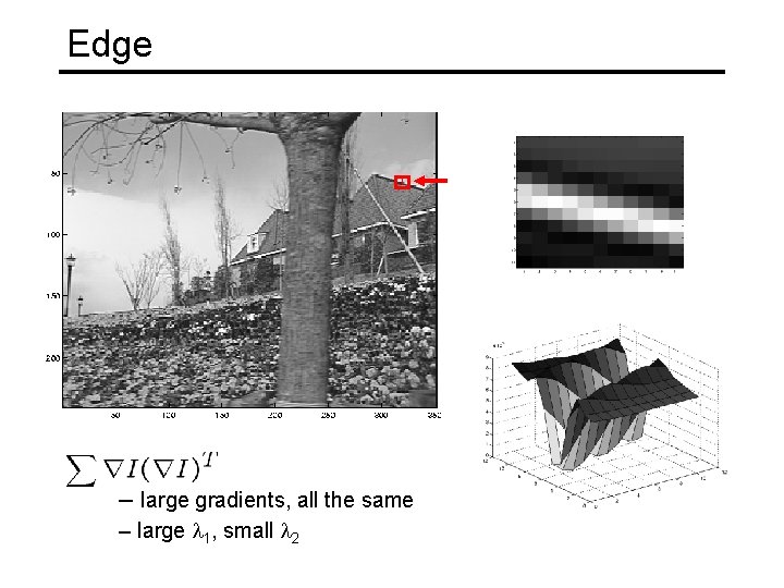
Eigenvectors of ATA Suppose (x, y) is on an edge. What is ATA? • gradients along edge all point the same direction • gradients away from edge have small magnitude • is an eigenvector with eigenvalue • What’s the other eigenvector of ATA? – let N be perpendicular to – N is the second eigenvector with eigenvalue 0 The eigenvectors of ATA relate to edge direction and magnitude

Edge – large gradients, all the same – large l 1, small l 2

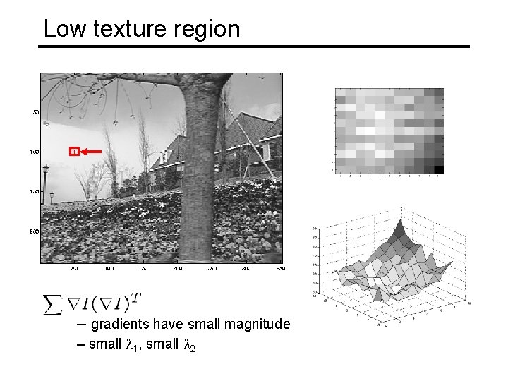
Low texture region – gradients have small magnitude – small l 1, small l 2

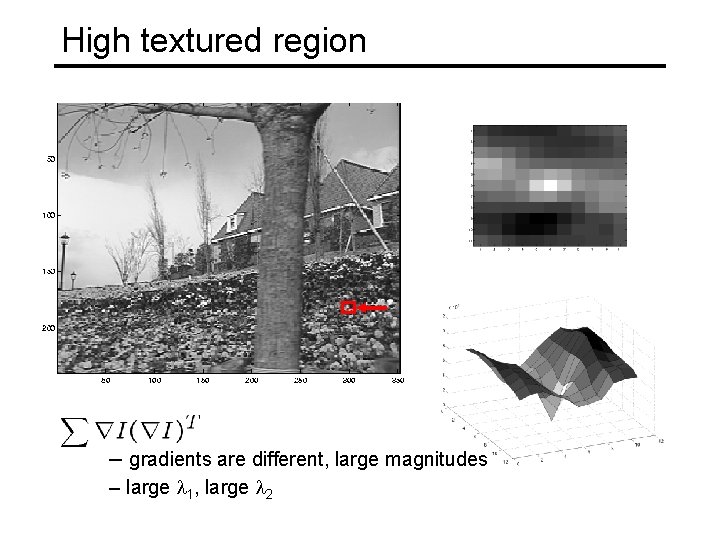
High textured region – gradients are different, large magnitudes – large l 1, large l 2

Observation This is a two image problem BUT • Can measure sensitivity by just looking at one of the images! • This tells us which pixels are easy to track, which are hard – very useful later on when we do feature tracking. . .

Errors in Lukas-Kanade What are the potential causes of errors in this procedure? • Suppose ATA is easily invertible • Suppose there is not much noise in the image When our assumptions are violated • Brightness constancy is not satisfied • The motion is not small • A point does not move like its neighbors – window size is too large – what is the ideal window size?

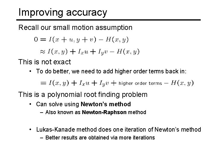
Improving accuracy Recall our small motion assumption This is not exact • To do better, we need to add higher order terms back in: This is a polynomial root finding problem • Can solve using Newton’s method – Also known as Newton-Raphson method • Lukas-Kanade method does one iteration of Newton’s method – Better results are obtained via more iterations

Iterative Refinement Iterative Lukas-Kanade Algorithm 1. Estimate velocity at each pixel by solving Lucas-Kanade equations 2. Warp H towards I using the estimated flow field - use image warping techniques 3. Repeat until convergence

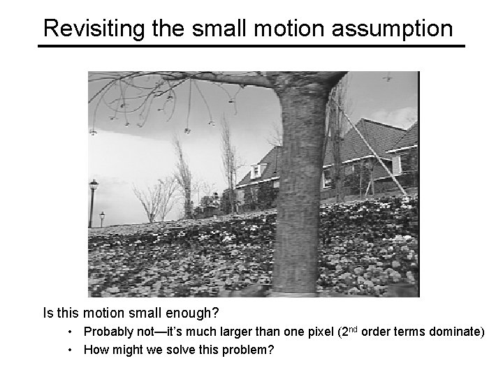
Revisiting the small motion assumption Is this motion small enough? • Probably not—it’s much larger than one pixel (2 nd order terms dominate) • How might we solve this problem?

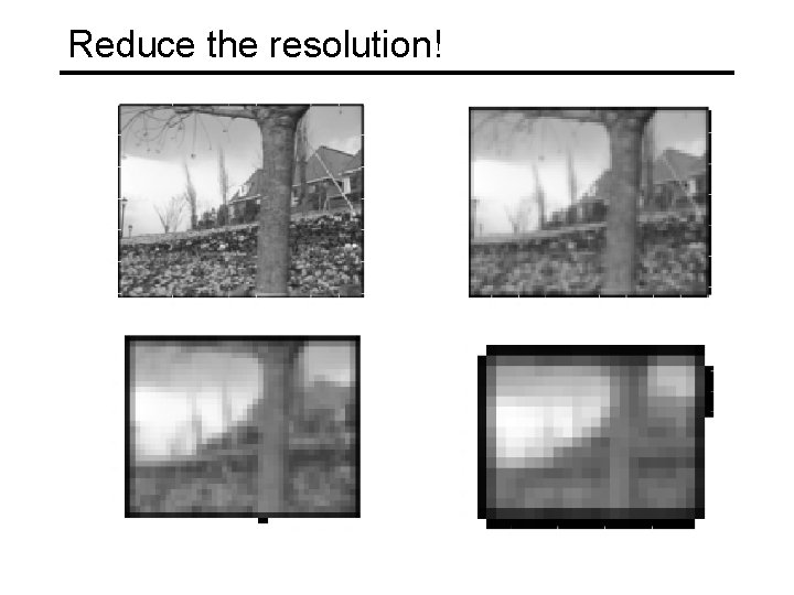
Reduce the resolution!

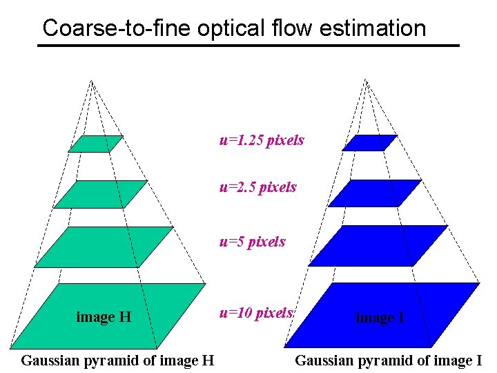
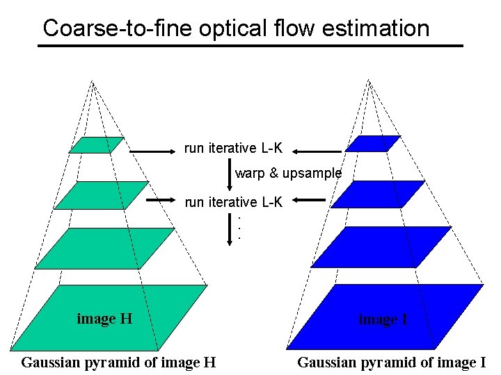
Coarse-to-fine optical flow estimation u=1. 25 pixels u=2. 5 pixels u=5 pixels image H Gaussian pyramid of image H u=10 pixels image I Gaussian pyramid of image I

Coarse-to-fine optical flow estimation run iterative L-K warp & upsample run iterative L-K. . . image H J Gaussian pyramid of image H image I Gaussian pyramid of image I

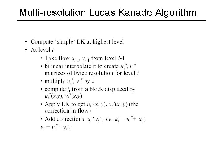
Multi-resolution Lucas Kanade Algorithm

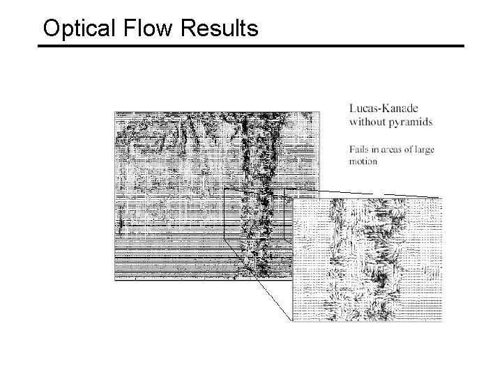
Optical Flow Results

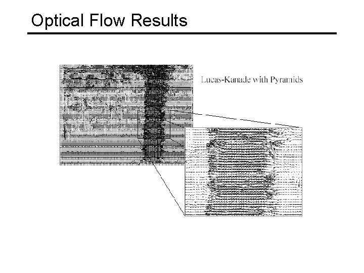
Optical Flow Results

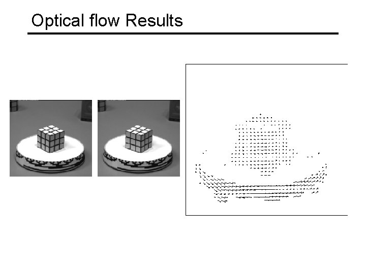
Optical flow Results

Suggested Readings • Chapter 8, Emanuele Trucco, Alessandro Verri, “Introductory Techniques for 3 -D Computer Vision”