Motion Estimation Uses of Motion 3 D shape

Motion Estimation Uses of Motion • 3 D shape reconstruction • Segment objects based on motion cues • Recognize events and activities • Improve video quality • Track objects • Correct for camera jitter (stabilization) • Align images (mosaics) • Efficient video representations • Video compression (e. g. , MPEG 2) • Special effects …

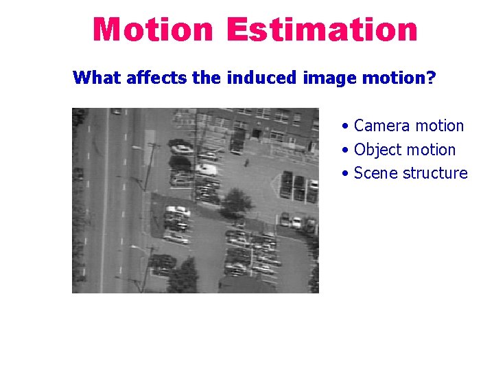
Motion Estimation What affects the induced image motion? • Camera motion • Object motion • Scene structure

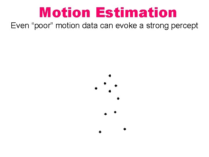
Motion Estimation Even “poor” motion data can evoke a strong percept

Motion Estimation Even “poor” motion data can evoke a strong percept

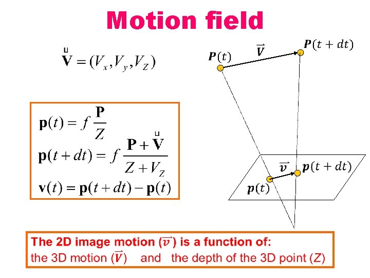
Motion field

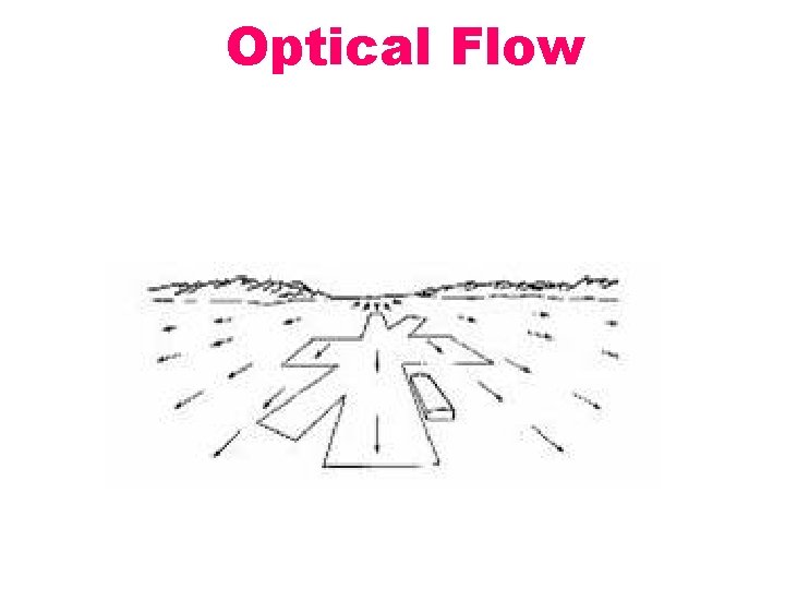
Optical Flow

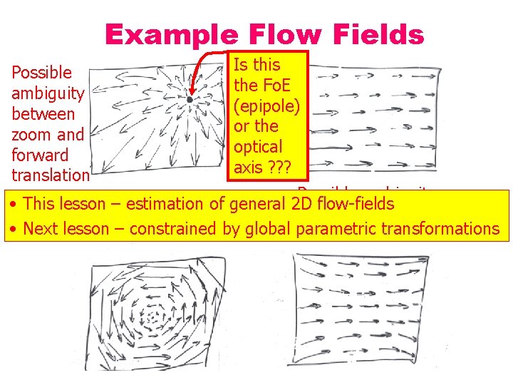
Example Flow Fields Possible ambiguity between zoom and forward translation Is this the Fo. E (epipole) or the optical axis ? ? ? Possible ambiguity • This lesson – estimation of general 2 D flow-fields between sideways • Next lesson – constrained by global parametric transformations translation and rotation

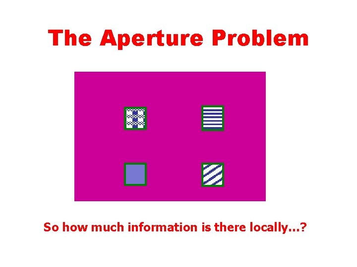
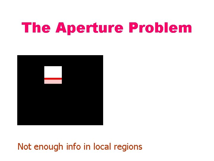
The Aperture Problem So how much information is there locally…?

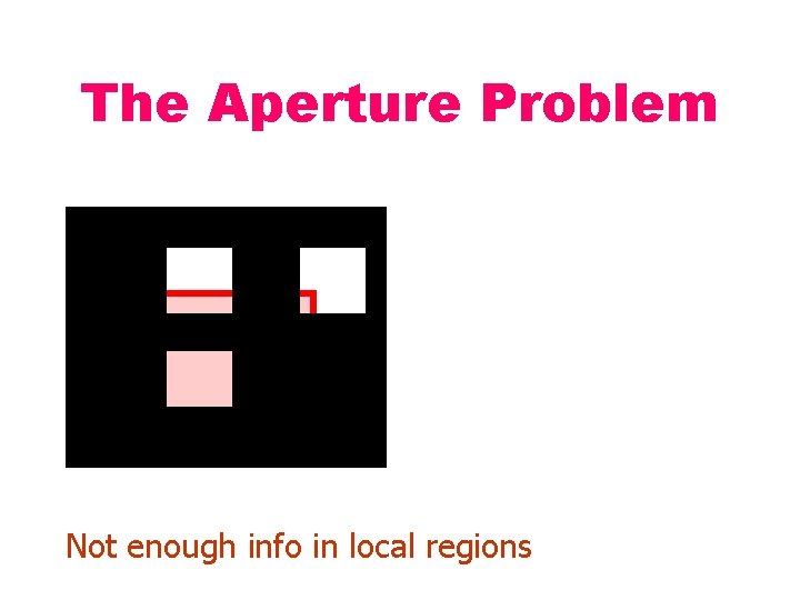
The Aperture Problem Not enough info in local regions Copyright, 1996 © Dale Carnegie & Associates, Inc.

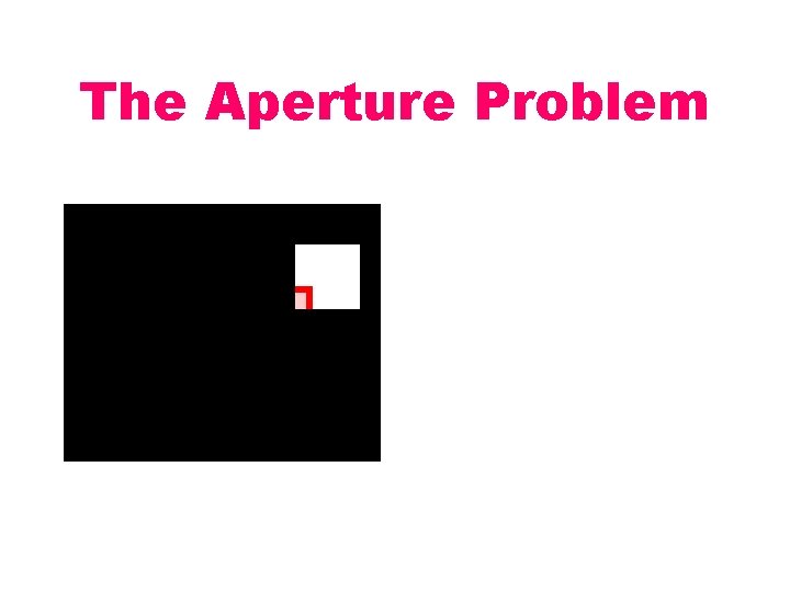
The Aperture Problem Not enough info in local regions Copyright, 1996 © Dale Carnegie & Associates, Inc.

The Aperture Problem Copyright, 1996 © Dale Carnegie & Associates, Inc.

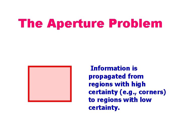
The Aperture Problem Information is propagated from regions with high certainty (e. g. , corners) to regions with low certainty. Copyright, 1996 © Dale Carnegie & Associates, Inc.

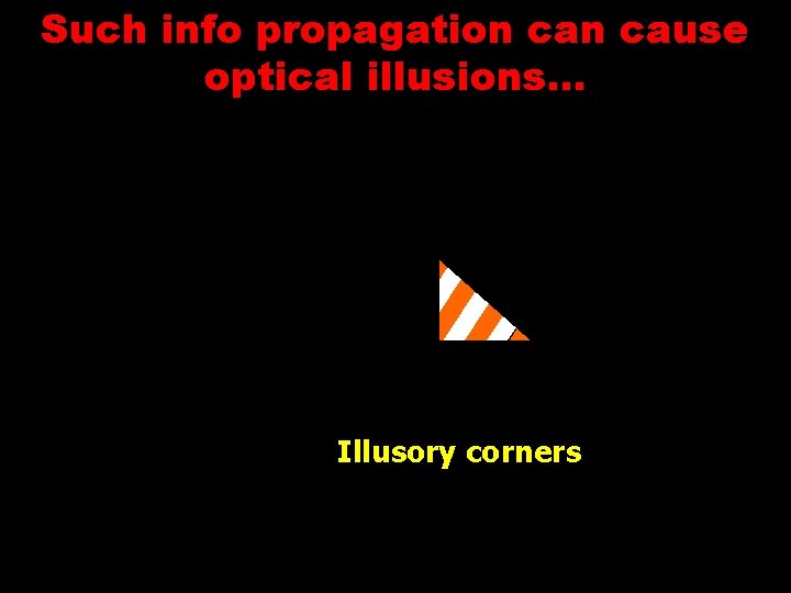
Such info propagation cause optical illusions… Illusory corners

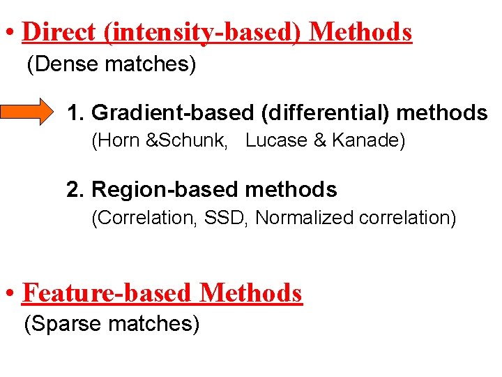
• Direct (intensity-based) Methods (Dense matches) 1. Gradient-based (differential) methods (Horn &Schunk, Lucase & Kanade) 2. Region-based methods (Correlation, SSD, Normalized correlation) • Feature-based Methods (Sparse matches)

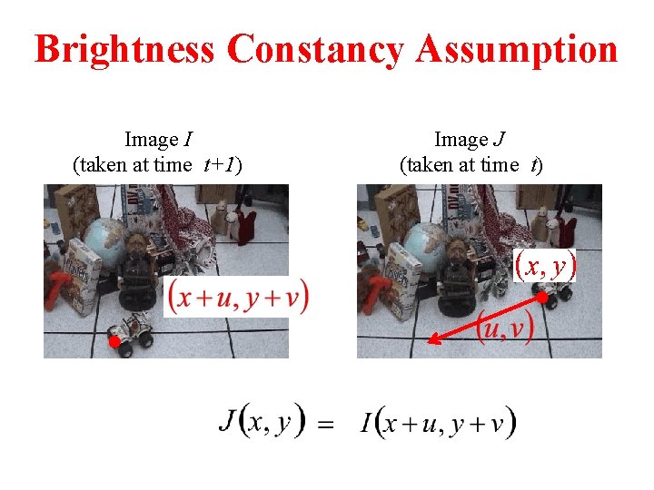
Brightness Constancy Assumption Image I (taken at time t+1) Image J (taken at time t)

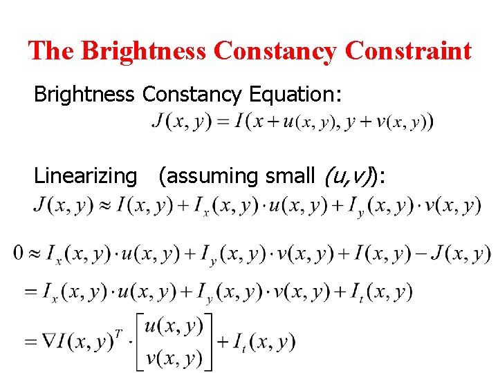
The Brightness Constancy Constraint Brightness Constancy Equation: Linearizing (assuming small (u, v)):

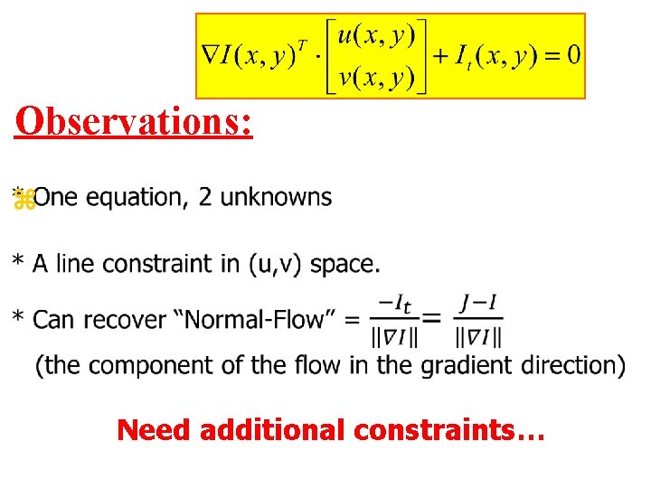
Observations: z Need additional constraints…

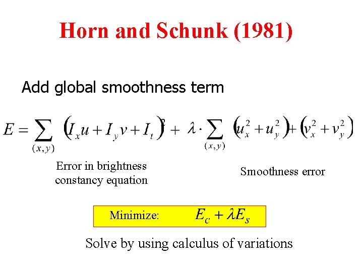
Horn and Schunk (1981) Add global smoothness term Error in brightness constancy equation Smoothness error Minimize: Solve by using calculus of variations

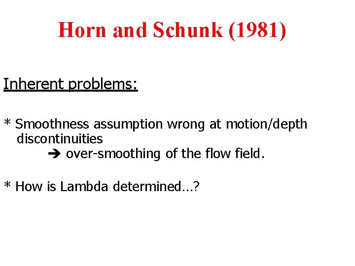
Horn and Schunk (1981) Inherent problems: * Smoothness assumption wrong at motion/depth discontinuities over-smoothing of the flow field. * How is Lambda determined…?

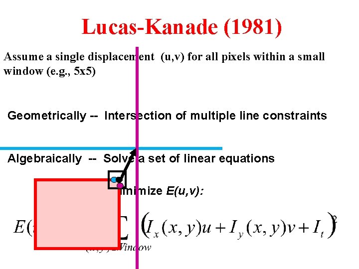
Lucas-Kanade (1981) Assume a single displacement (u, v) for all pixels within a small window (e. g. , 5 x 5) Geometrically -- Intersection of multiple line constraints Algebraically -- Solve a set of linear equations Minimize E(u, v):

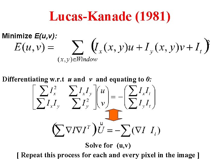
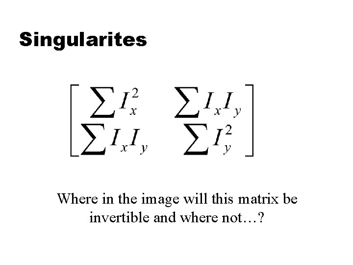
Lucas-Kanade (1981) Minimize E(u, v): Differentiating w. r. t u and v and equating to 0: Solve for (u, v) [ Repeat this process for each and every pixel in the image ]

Singularites Where in the image will this matrix be invertible and where not…?

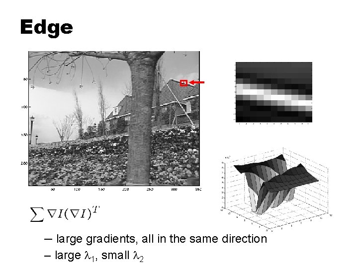
Edge – large gradients, all in the same direction – large l 1, small l 2

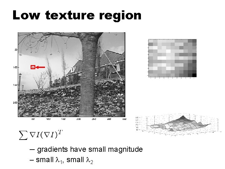
Low texture region – gradients have small magnitude – small l 1, small l 2

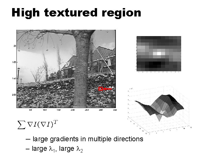
High textured region – large gradients in multiple directions – large l 1, large l 2

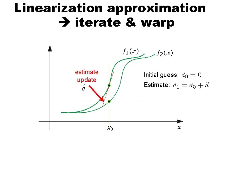
Linearization approximation iterate & warp estimate update Initial guess: Estimate: x 0 x

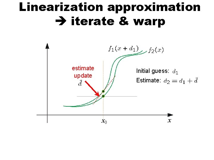
Linearization approximation iterate & warp + estimate update Initial guess: Estimate: x 0 x

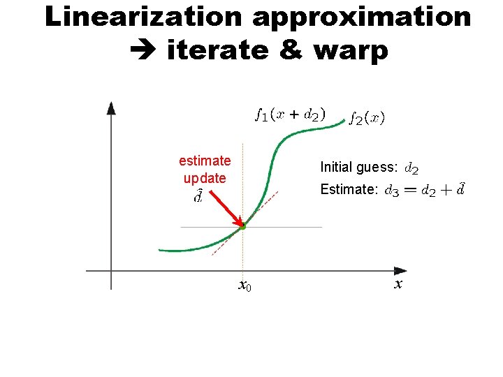
Linearization approximation iterate & warp + estimate update Initial guess: Estimate: x 0 x

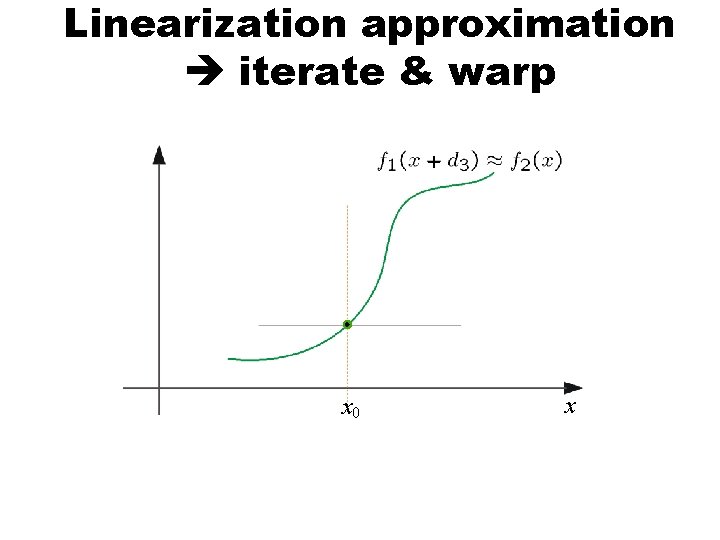
Linearization approximation iterate & warp + x 0 x

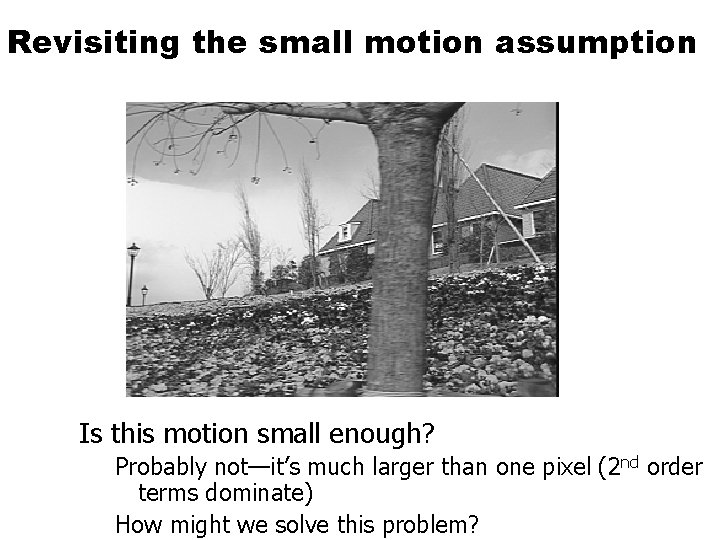
Revisiting the small motion assumption Is this motion small enough? Probably not—it’s much larger than one pixel (2 nd order terms dominate) How might we solve this problem?

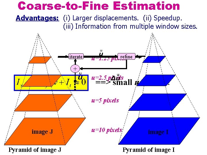
Coarse-to-Fine Estimation Advantages: (i) Larger displacements. (ii) Speedup. (iii) Information from multiple window sizes. iterate refine u=1. 25 pixels + u=2. 5 pixels ==> small u and v. . . u=5 pixels image J Pyramid of image J u=10 pixels image I Pyramid of image I

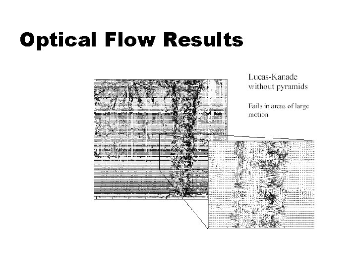
Optical Flow Results

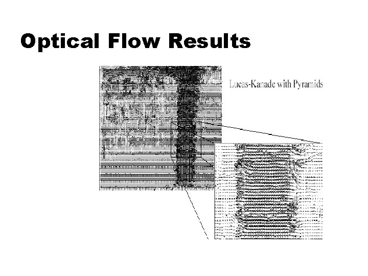
Optical Flow Results

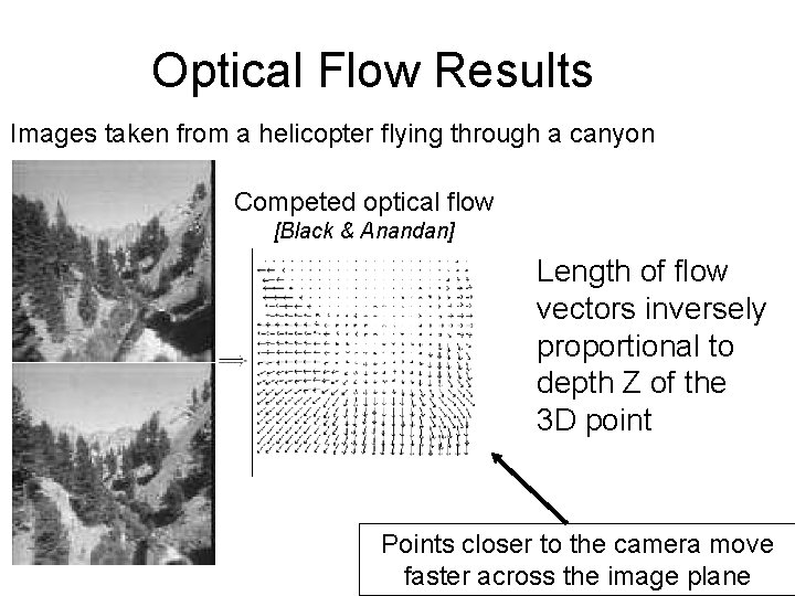
Optical Flow Results Images taken from a helicopter flying through a canyon Competed optical flow [Black & Anandan] Length of flow vectors inversely proportional to depth Z of the 3 D point Points closer to the camera move faster across the image plane

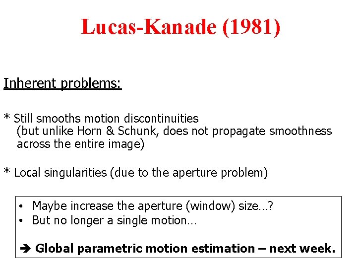
Lucas-Kanade (1981) Inherent problems: * Still smooths motion discontinuities (but unlike Horn & Schunk, does not propagate smoothness across the entire image) * Local singularities (due to the aperture problem) • Maybe increase the aperture (window) size…? • But no longer a single motion… Global parametric motion estimation – next week.

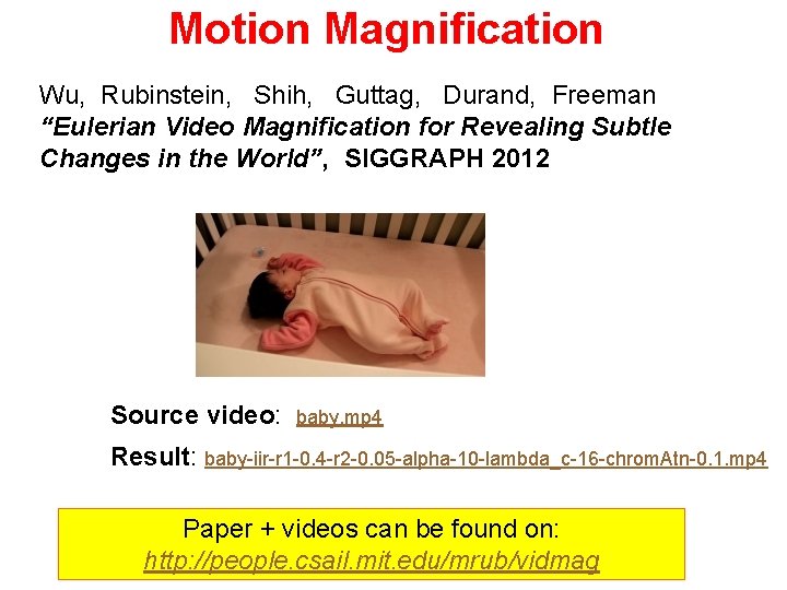
Motion Magnification Wu, Rubinstein, Shih, Guttag, Durand, Freeman “Eulerian Video Magnification for Revealing Subtle Changes in the World”, SIGGRAPH 2012 Source video: baby. mp 4 Result: baby-iir-r 1 -0. 4 -r 2 -0. 05 -alpha-10 -lambda_c-16 -chrom. Atn-0. 1. mp 4 Paper + videos can be found on: http: //people. csail. mit. edu/mrub/vidmag

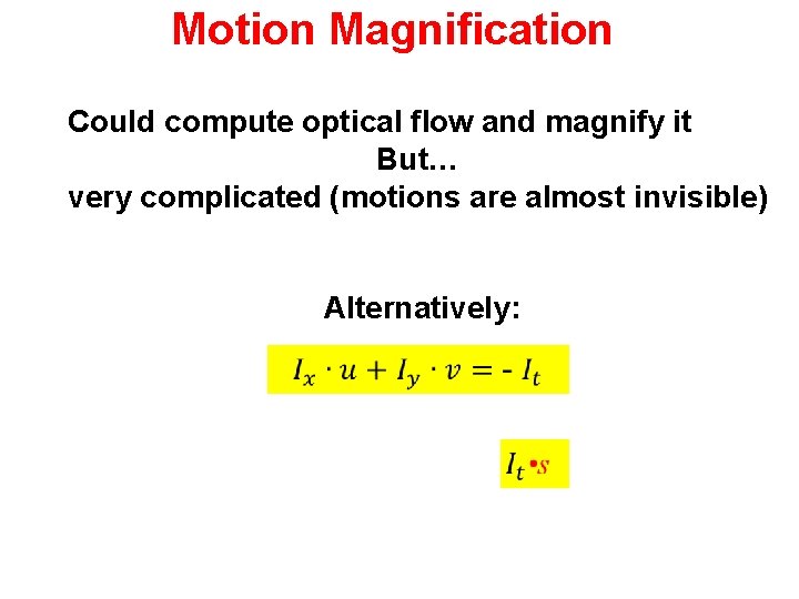
Motion Magnification Could compute optical flow and magnify it But… very complicated (motions are almost invisible) Alternatively:

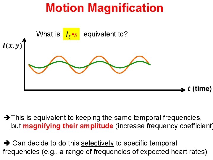
Motion Magnification What is equivalent to? This is equivalent to keeping the same temporal frequencies, but magnifying their amplitude (increase frequency coefficient) Can decide to do this selectively to specific temporal frequencies (e. g. , a range of frequencies of expected heart rates).

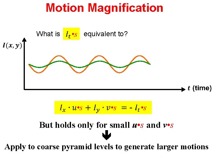
Motion Magnification What is equivalent to? But holds only for small u • s and v • s Apply to coarse pyramid levels to generate larger motions

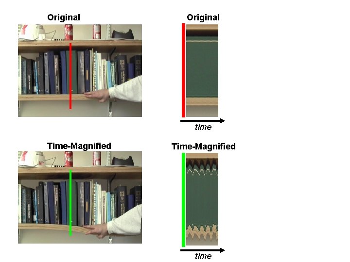
Original time Time-Magnified time

Motion Magnification Paper + videos can be found on: http: //people. csail. mit. edu/mrub/vidmag EVM_NSFSci. Vis 2012. mov Copyright, 1996 © Dale Carnegie & Associates, Inc.

Motion Magnification Paper + videos can be found on: http: //people. csail. mit. edu/mrub/vidmag. mov