More on the FermiDirac Distribution Plus Some Brief

More on the Fermi-Dirac Distribution Plus Some Brief History!
 Statistics in 1926, understanding some aspects")
• Before the introduction of Fermi–Dirac (FD) Statistics in 1926, understanding some aspects of electron behavior was lacking due to seemingly contradictory phenomena. Example: • The electronic Heat Capacity of a metal at Room Temperature seemed to come from 100 Times Fewer Electrons (!) than were in the electric current!!

• It was also not understood why Emission Currents, generated by applying high electric fields to metals at room temperature, were almost independent of temperature.

• A problem with the electronic theory of metals at that time was due to considering that The electrons were (according to classical statistical mechanics) all equivalent. • That is, it was believed that each electron contributed to the specific heat an amount on the order of the Boltzmann constant k (On the basis of the Equipartition Theorem).
 of FD")
• These problems remained unsolved until the after discovery (invention? ) of FD statistics. FD Statistics was first Published in 1926 by Enrico Fermi and P. A. M. Dirac.

FD Statistics: Published in 1926 • Science historians have said that, actually, in 1925, Pascual Jordan developed what is now known as FD Statistics! • He called his theory “Pauli Statistics”. But, he didn’t publish right away for some reason. (A lesson for those of you who want to do research!)

FD Statistics: Published in 1926 • According to Dirac, FD Statistics was first studied by Fermi. • Dirac called theory “Fermi Statistics” & the corresponding particles he called “Fermions”.

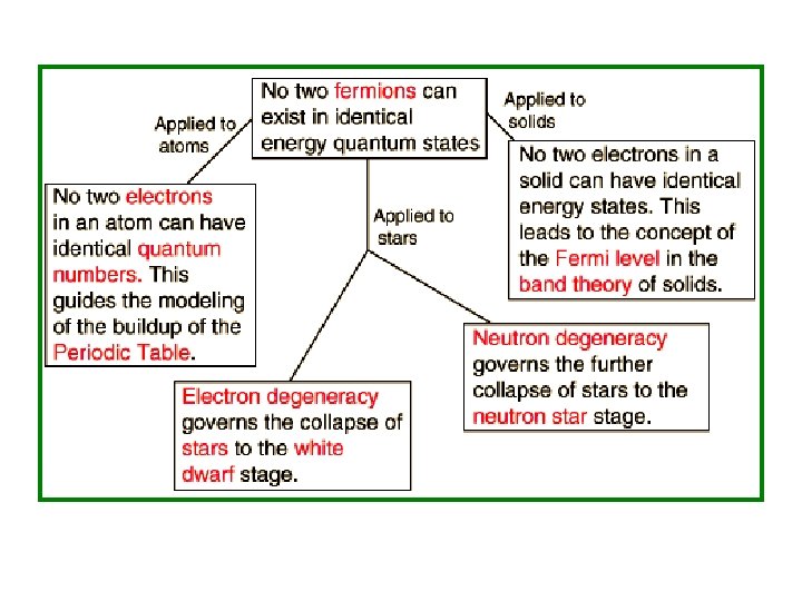
• 1926: Fowler applied FD Statistics to describe the collapse of a star to a white dwarf. • 1927: Sommerfeld applied it to electrons in metals. • 1928: Fowler & Nordheim applied it to field electron emission from metals. FD Statistics is obviously still a very important part of physics!

More FD & BE Statistics Discussion • The occupation numbers, or the number n of particles allowed in each one-particle quantum state are restricted by a principle of many body quantum mechanics: • The Many Body Wave Function Ψ of a system of identical particles has the following property: For Bosons • If 2 particles exchange all quantum numbers Ψ must be Symmetric (no sign change): Ψ' = Ψ

More FD & BE Statistics Discussion • The occupation numbers, or the number n of particles allowed in each one-particle quantum state is restricted by a principle of many body quantum mechanics: • The Many Body Wave Function Ψ of a system of identical particles has the following property: For Fermions • If 2 particles exchange all quantum numbers Ψ must be Antisymmetric (sign change): Ψ' = -Ψ

Bosons: Ψ is Symmetric when 2 particles exchange all quantum numbers. Ψ' = Ψ • It can be shown that for Bosons, this means that the occupation number n can be 0 or any positive integer: n = 0, 1, 2, 3. . .

Fermions: Ψ is Antisymmetric when 2 particles exchange all quantum numbers. Ψ' = -Ψ • It can be shown that for Fermions, this means that the occupation number n is restricted to 0 or 1!! n = 0 or 1 ONLY!

• The differences between Bosons & Fermions are determined by the nature of the particles. Particles which obey Fermi-Dirac Statistics are called Fermi-Particles Fermions They have spin S = (½)*(odd integer)ħ • Examples: Electrons, Positrons, Protons, Neutrons, Quarks, ….

• The differences between Bosons & Fermions are determined by the nature of the particles. Particles which obey Bose-Einstein Statistics are called Bose-Particles Bosons These have spin S = (integer)*(ħ) • Examples: 4 Photons, Phonons, He, . .

Consider Fermions & Bosons in a 1 -D Potential Well
 • In a System of N Fermions: 2 of")
Wolfgang Pauli Exclusion Principle (Fermions) • In a System of N Fermions: 2 of them can’t occupy the same single particle state. Or: No 2 of them can have exactly the same set of quantum numbers. Example • A 2 Fermion, Antisymmetric Wave. Function • 2 Electrons, a & b • 2 atomic states, 1 & 2. • 2 Wave Functions ψ1(a) & ψ2(b) See Figure
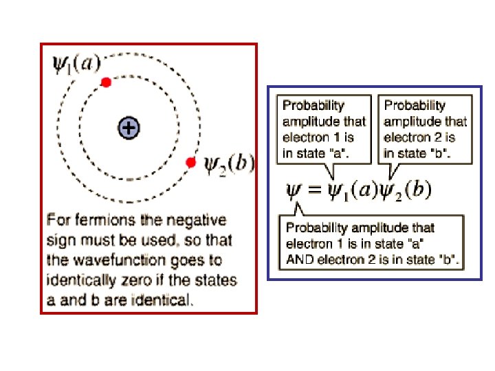

Symmetric & Antisymmetric Wave Functions Further Discussion • Consider 2 Identical Particles (1 & 2) which may exist in 2 Different States (a & b). • To construct a Wave Function for the 2 particle system, 2 separate possibilities come to mind: and • If the particles are indistinguishable, we can’t tell whether the 2 particle system is in state I or II. Both are equally likely, so we write The system wave function as a linear combination of I & II.

• If the Particles are Bosons, the 2 particle wave function must be Symmetric: • If the Particles are Fermions, the 2 particle wave function must be Antisymmetric:

• What happens if we try to put both particles 1 & 2 in the same state? If the particles are distinguishable, we can write: • The subscript M indicates Maxwell-Boltzmann statistics, because the particles are distinguishable. • The probability density for distinguishable particles is • Note: MB Statistics is for classical (not quantum) particles. So why the wave functions here? In this case, it is useful for comparing MB results with quantum statistics.

For Bosons: with probability density: or: • In other words if the particles are Bosons, they are twice as likely to be in the same state as distinguishable classical particles!

• On the other hand, For Fermions: with probability density: F* F = (½)[| a(1) a(2)|2 + | a(2) a(1)|2 - a(1) a(2) a(1) or: • In other words, If the particles are Fermions, the probability that they are in the same state is identically ZERO! The Pauli Exclusion Principle is “proven”!

• In general, the presence of a Boson in a particular quantum state increases the probability that other Bosons will be found in the same state… • However, the presence of a Fermion in a particular quantum state prevents other Fermions from being in that state.
")
The Fermi-Dirac Distribution Enrico Fermi 1901 - 1954 P. A. M. Dirac (5. 46) 1902 - 1984

Fermi-Dirac Distribution: Summary of the physics of this distribution • Consider a system of identical, independent, non -interacting particles in a common volume V & obeying anti-symmetric statistics: That is, spin = (½)nħ, n = odd integer. • According to the Pauli Principle, the total many particle wave function is anti-symmetric on interchange of any two particles. • Because the particles are non-interacting, it is convenient to discuss the system in terms of the energy states i of one particle in a volume V.

• Specify the system state by specifying the number of particles ni , occupying the eigenstate of energy i. i denotes a single state. • The Pauli principle allows only the values ni = 1, 0. 0 This is, of course, the elementary statement of The Pauli Principle: A given single-particle state may not be occupied by more than one identical particle.
,")
Fermi-Dirac Distribution Function. • This distribution is often written in terms of f( ), where f is the probability that a state of energy is occupied: • It is implicit in the derivation of f(ε) that is the chemical potential. Often is called the Fermi Level, or, for the free electron gas, the Fermi Energy EF.
/k.")
Classical Limit • For sufficiently large , it is true that ( - )/k. T >>1 & in this limit • This is just the Maxwell-Boltzmann (MB) Distribution. So, the high-energy tail of the Fermi-Dirac Distribution is similar to the MB Distribution. • The condition for the approximate validity of the MB Distribution for all energies 0 is that

The Bose-Einstein Distribution S. N. Bose 1894 - 1974 Albert Einstein 1894 - 1954 We’ll discuss some of the physics of this distribution soon.
- Slides: 30