More Dynamic Programming FloydWarshall Algorithm Announcements Ill try

More Dynamic Programming Floyd-Warshall Algorithm

Announcements I’ll try to post Assignment #5 (the last one!) either tonight or tomorrow. Assignment #4 is due next Monday The Final is on Monday Dec. 13 4 pm- 6 pm. Same room. Not 4: 30 pm!!

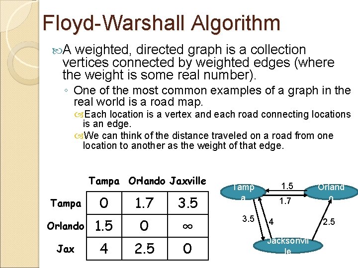
Floyd-Warshall Algorithm A weighted, directed graph is a collection vertices connected by weighted edges (where the weight is some real number). ◦ One of the most common examples of a graph in the real world is a road map. Each location is a vertex and each road connecting locations is an edge. We can think of the distance traveled on a road from one location to another as the weight of that edge. Tampa Orlando Jaxville Tampa Orlando Jax 0 1. 5 4 1. 7 0 2. 5 3. 5 ∞ 0 1. 5 Tamp a 3. 5 1. 7 4 Jacksonvil le Orland o 2. 5

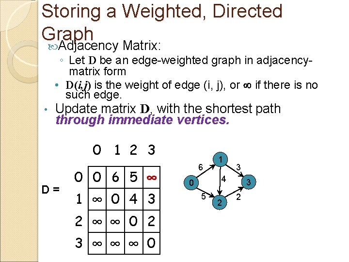
Storing a Weighted, Directed Graph Adjacency Matrix: ◦ Let D be an edge-weighted graph in adjacencymatrix form • D(i, j) is the weight of edge (i, j), or ¥ if there is no such edge. • Update matrix D, with the shortest path through immediate vertices. 0 1 2 3 D= 0 0 6 5 ∞ 1 ∞ 0 4 3 2 ∞ ∞ 0 2 3 ∞ ∞ ∞ 0 6 1 3 4 0 5 2 3 2

Floyd-Warshall Algorithm Given a weighted graph, we want to know the shortest path from one vertex in the graph to another. ◦ The Floyd-Warshall algorithm determines the shortest path between all pairs of vertices in a graph. ◦ What is the difference between Floyd. Warshall and Dijkstra’s? ?

Floyd-Warshall Algorithm If V is the number of vertices, Dijkstra’s runs in (V 2) ◦ We could just call Dijkstra |V| times, passing a different source vertex each time. ◦ (V V 2) = (V 3) ◦ (Which is the same runtime as the Floyd. Warshall Algorithm) BUT, Dijkstra’s doesn’t work with negative-weight edges.

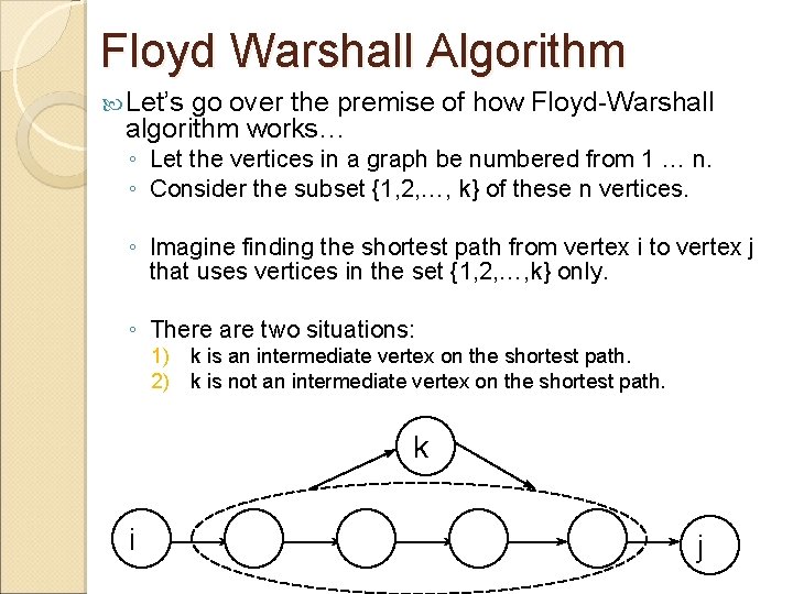
Floyd Warshall Algorithm Let’s go over the premise of how Floyd-Warshall algorithm works… ◦ Let the vertices in a graph be numbered from 1 … n. ◦ Consider the subset {1, 2, …, k} of these n vertices. ◦ Imagine finding the shortest path from vertex i to vertex j that uses vertices in the set {1, 2, …, k} only. ◦ There are two situations: 1) k is an intermediate vertex on the shortest path. 2) k is not an intermediate vertex on the shortest path. k i j

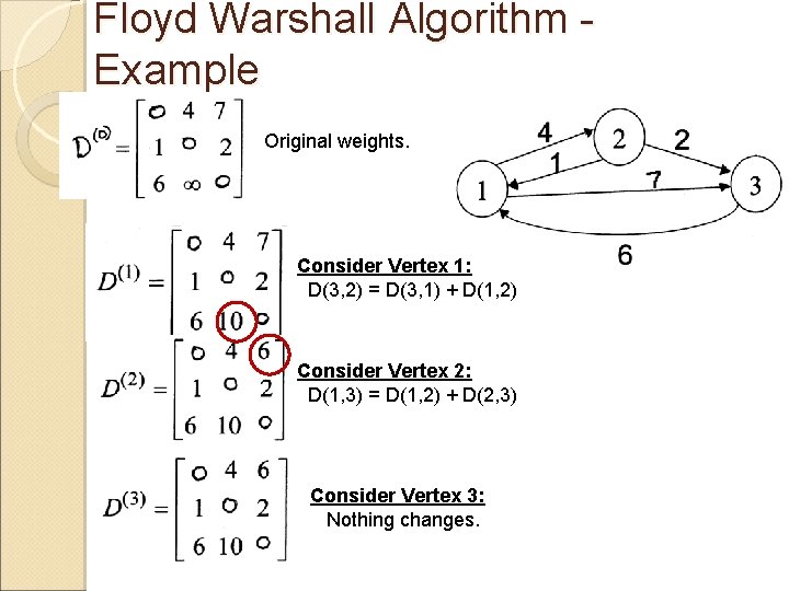
Floyd Warshall Algorithm - Example Original weights. Consider Vertex 1: D(3, 2) = D(3, 1) + D(1, 2) Consider Vertex 2: D(1, 3) = D(1, 2) + D(2, 3) Consider Vertex 3: Nothing changes.

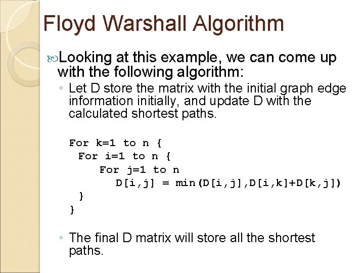
Floyd Warshall Algorithm Looking at this example, we can come up with the following algorithm: ◦ Let D store the matrix with the initial graph edge information initially, and update D with the calculated shortest paths. For k=1 to n { For i=1 to n { For j=1 to n D[i, j] = min(D[i, j], D[i, k]+D[k, j]) } } ◦ The final D matrix will store all the shortest paths.

Floyd Warshall Algorithm Example on the board…

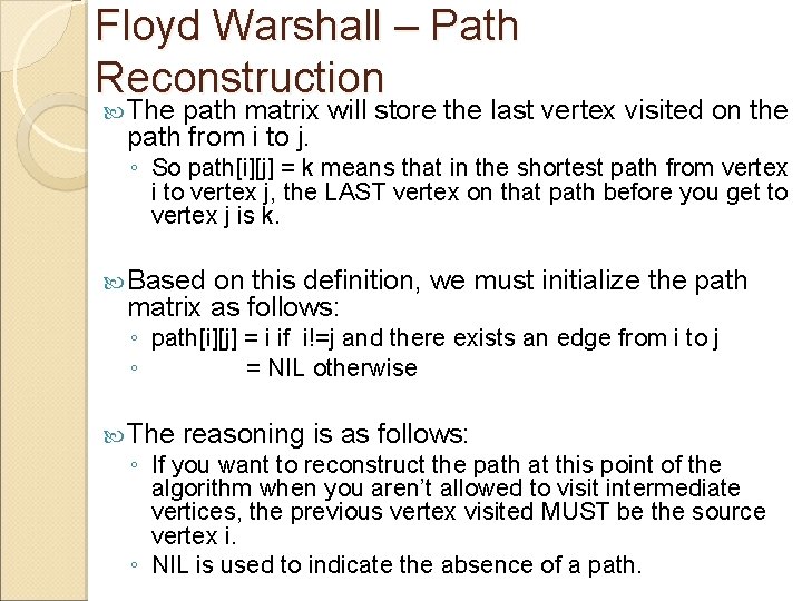
Floyd Warshall – Path Reconstruction The path matrix will store the last vertex visited on the path from i to j. ◦ So path[i][j] = k means that in the shortest path from vertex i to vertex j, the LAST vertex on that path before you get to vertex j is k. Based on this definition, we must initialize the path matrix as follows: ◦ path[i][j] = i if i!=j and there exists an edge from i to j ◦ = NIL otherwise The reasoning is as follows: ◦ If you want to reconstruct the path at this point of the algorithm when you aren’t allowed to visit intermediate vertices, the previous vertex visited MUST be the source vertex i. ◦ NIL is used to indicate the absence of a path.

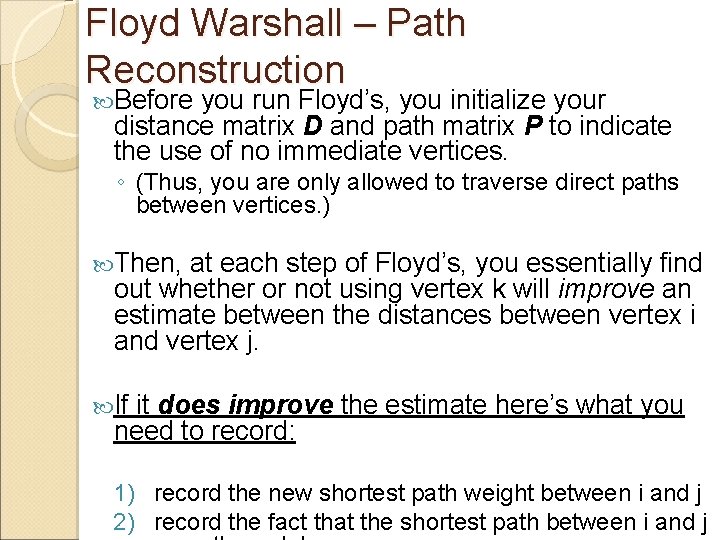
Floyd Warshall – Path Reconstruction Before you run Floyd’s, you initialize your distance matrix D and path matrix P to indicate the use of no immediate vertices. ◦ (Thus, you are only allowed to traverse direct paths between vertices. ) Then, at each step of Floyd’s, you essentially find out whether or not using vertex k will improve an estimate between the distances between vertex i and vertex j. If it does improve the estimate here’s what you need to record: 1) record the new shortest path weight between i and j 2) record the fact that the shortest path between i and j

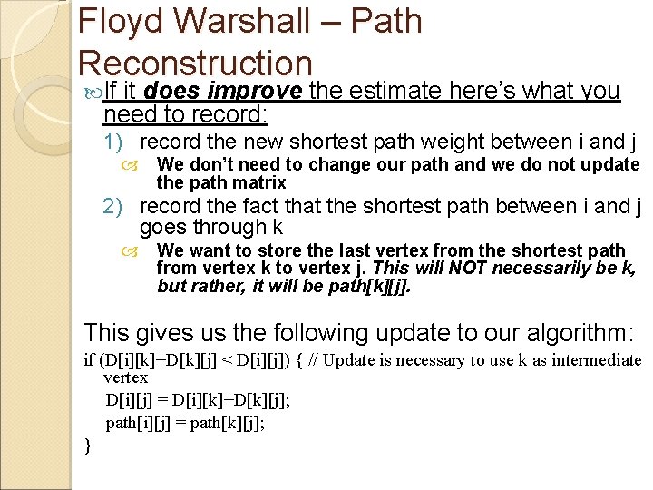
Floyd Warshall – Path Reconstruction If it does improve the estimate here’s what you need to record: 1) record the new shortest path weight between i and j We don’t need to change our path and we do not update the path matrix 2) record the fact that the shortest path between i and j goes through k We want to store the last vertex from the shortest path from vertex k to vertex j. This will NOT necessarily be k, but rather, it will be path[k][j]. This gives us the following update to our algorithm: if (D[i][k]+D[k][j] < D[i][j]) { // Update is necessary to use k as intermediate vertex D[i][j] = D[i][k]+D[k][j]; path[i][j] = path[k][j]; }

Path Reconstruction Example on the board…

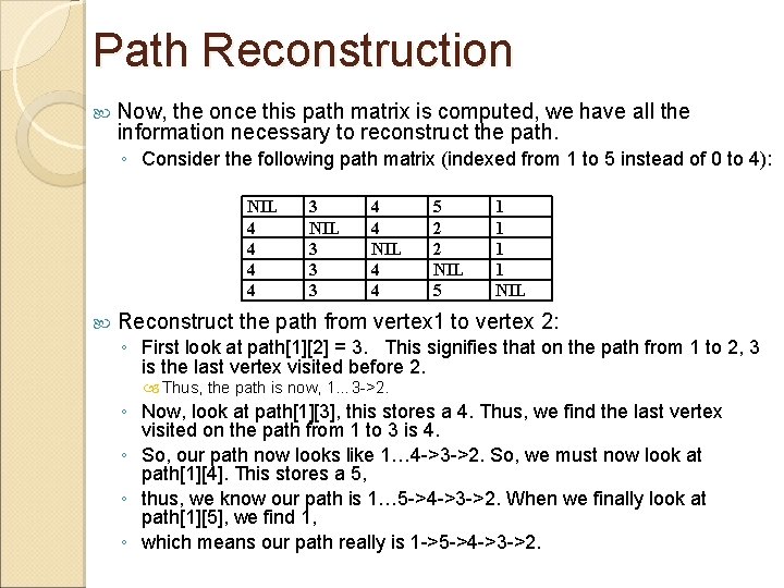
Path Reconstruction Now, the once this path matrix is computed, we have all the information necessary to reconstruct the path. ◦ Consider the following path matrix (indexed from 1 to 5 instead of 0 to 4): NIL 4 4 3 NIL 3 3 3 4 4 NIL 4 4 5 2 2 NIL 5 1 1 NIL Reconstruct the path from vertex 1 to vertex 2: ◦ First look at path[1][2] = 3. This signifies that on the path from 1 to 2, 3 is the last vertex visited before 2. Thus, the path is now, 1… 3 ->2. ◦ Now, look at path[1][3], this stores a 4. Thus, we find the last vertex visited on the path from 1 to 3 is 4. ◦ So, our path now looks like 1… 4 ->3 ->2. So, we must now look at path[1][4]. This stores a 5, ◦ thus, we know our path is 1… 5 ->4 ->3 ->2. When we finally look at path[1][5], we find 1, ◦ which means our path really is 1 ->5 ->4 ->3 ->2.

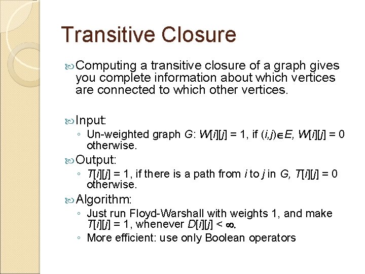
Transitive Closure Computing a transitive closure of a graph gives you complete information about which vertices are connected to which other vertices. Input: ◦ Un-weighted graph G: W[i][j] = 1, if (i, j)ÎE, W[i][j] = 0 otherwise. Output: ◦ T[i][j] = 1, if there is a path from i to j in G, T[i][j] = 0 otherwise. Algorithm: ◦ Just run Floyd-Warshall with weights 1, and make T[i][j] = 1, whenever D[i][j] < ¥. ◦ More efficient: use only Boolean operators

Transitive Closure Transitive-Closure(W[1. . n]) 01 T ¬ W // T(0) 02 for k ¬ 1 to n do // compute T(k) 03 for i ¬ 1 to n do 04 for j ¬ 1 to n do 05 T[i][j] ¬ T[i][j] Ú (T[i][k] Ù T[k][j]) 06 return T This is the SAME as the other Floyd-Warshall Algorithm, except for when we find a non-infinity estimate, we simply add an edge to the transitive closure graph. Every round we build off the previous paths reached. ◦ After iterating through all vertices being intermediate vertices, we have tried to connect all pairs of vertices i and j through all intermediate vertices k.

Transitive Closure Example on the board…

References Slides adapted from Arup Guha’s Computer Science II Lecture notes: http: //www. cs. ucf. edu/~dmarino/ucf/cop 350 3/lectures/ Additional material from the textbook: Data Structures and Algorithm Analysis in Java (Second Edition) by Mark Allen Weiss Additional images: www. wikipedia. com xkcd. com