MONTE CARLO METHODS INTEGRATION and SAMPLING TECHNIQUES Monte

MONTE` CARLO METHODS INTEGRATION and SAMPLING TECHNIQUES Monte` Carlo Methods 1

THE BOOK by THE MAN Monte` Carlo Methods 2

PROBLEM STATEMENT • System of equations and inequalities defines a region in m-space • Determine the volume of the region Monte` Carlo Methods 3

HISTORY • 19 th C. simple integral like E[X] using straight-forward sampling • System of PDE solved using sample paths of Markov Chains – Rayleigh 1899 – Markov 1931 • Particles through a medium solved using Poisson Process and Random Walk – Manhattan Project • Combinatorics in the ’ 80’s in RTP, NC Monte` Carlo Methods 4

GROOMING • R = volumetric region • R confined to [0, 1]m • l(R) = volume • Generalized area-under-thecurve problem Monte` Carlo Methods 5

ALGORITHM • for i=1 to n – generate x in [0, 1]m – is x in R? • S=S+1 • end • l(R)=S/n Monte` Carlo Methods 6

MESH • Generate x’s as a mesh of evenly spaced points • Each point is 1/k from its nearest neighbor • n=km • Many varieties of this method, generally called Multi-Grid Monte` Carlo Methods 7

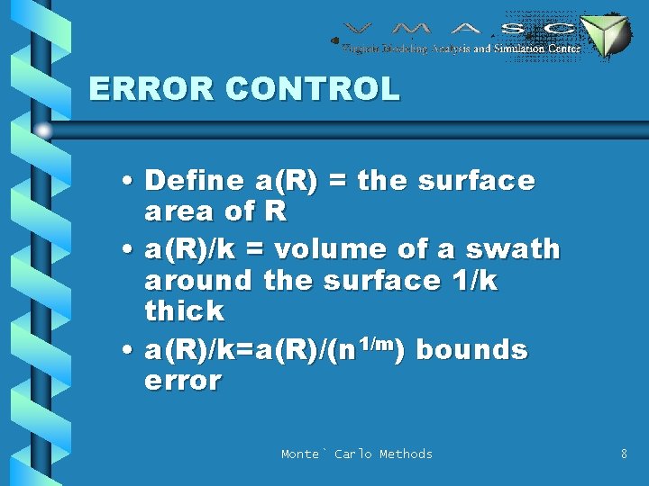
ERROR CONTROL • Define a(R) = the surface area of R • a(R)/k = volume of a swath around the surface 1/k thick • a(R)/k=a(R)/(n 1/m) bounds error Monte` Carlo Methods 8

. . . more ERROR CONTROL Monte` Carlo Methods 9

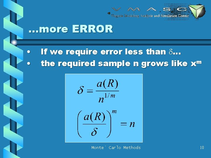
. . . more ERROR • • If we require error less than d. . . the required sample n grows like xm Monte` Carlo Methods 10

PROBABLY NOT THAT BAD • Reaction: the boundary of R isn’t usually so-aligned • Probability statement on the functions? – this math exists but is only marginally helpful with applied problems Monte` Carlo Methods 11

ALTERNATIVE • Monte` Carlo Method • for i = 1 to n – sample x from Uniform[0, 1]m – is x in R? • S = S + 1 • end • lhat = S/n Monte` Carlo Methods 12

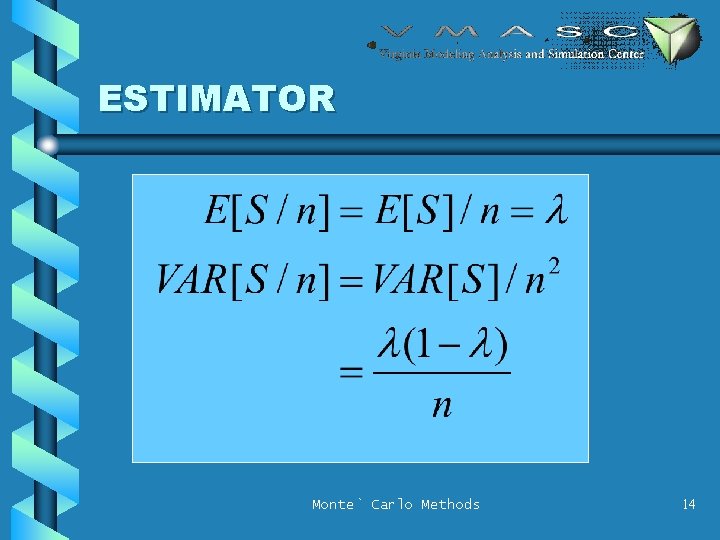
STATISTICAL TREATMENT • S is now a RANDOM VARIABLE • P[x in R] = l • • – (volume of R)/(volume of unit hyper-cube) S is a sum of Bernoulli Trials S is Binomial(n, l) E[S] = ln VAR[S] = n l (1 - l) Monte` Carlo Methods 13

ESTIMATOR Monte` Carlo Methods 14

CHEBYCHEV’S INEQUALITY • Bounds Tails of Distributions • Z~F, E[Z]=0, VAR[Z]= s 2, b>0 Monte` Carlo Methods 15

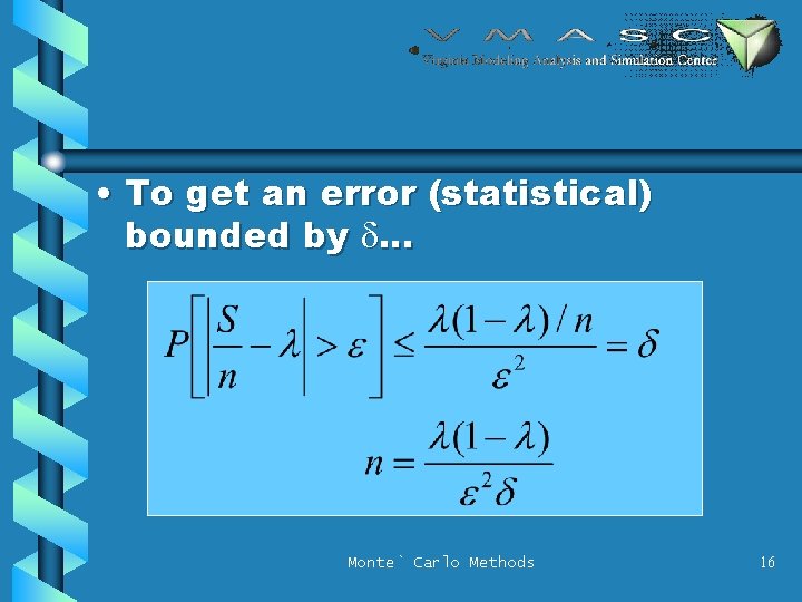
• To get an error (statistical) bounded by d. . . Monte` Carlo Methods 16

SIMPLER BOUNDS • l (1 - l) is bounded by ¼ • n = 1/(4 e 2 d) • Does not depend on m! Monte` Carlo Methods 17

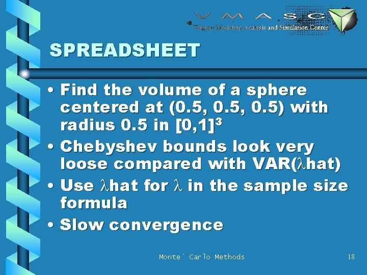
SPREADSHEET • Find the volume of a sphere centered at (0. 5, 0. 5) with radius 0. 5 in [0, 1]3 • Chebyshev bounds look very loose compared with VAR(lhat) • Use lhat for l in the sample size formula • Slow convergence Monte` Carlo Methods 18

STRATIFIED SAMPLING • Best of Mesh and Sampling Methods • Very General application of Variance Reduction – survey sampling – experimental design – optimization via simulation Monte` Carlo Methods 19

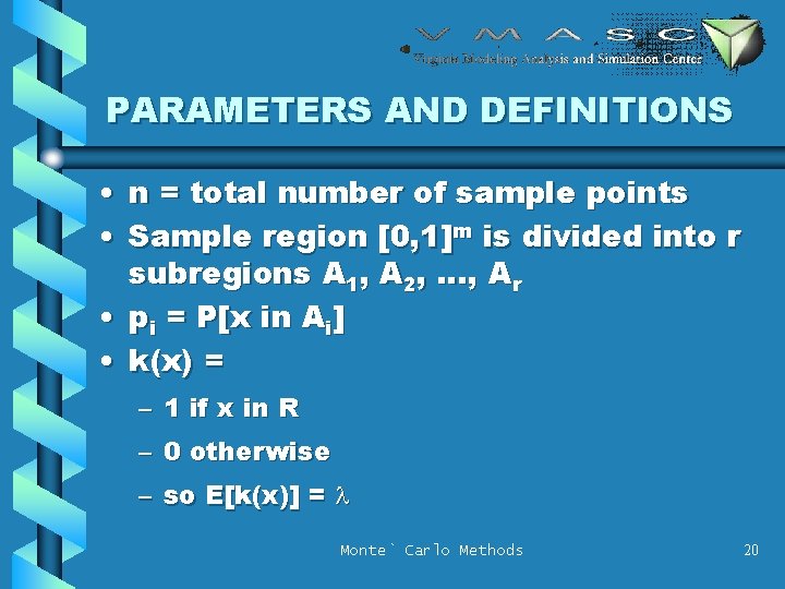
PARAMETERS AND DEFINITIONS • n = total number of sample points • Sample region [0, 1]m is divided into r subregions A 1, A 2, . . . , Ar • pi = P[x in Ai] • k(x) = – 1 if x in R – 0 otherwise – so E[k(x)] = l Monte` Carlo Methods 20

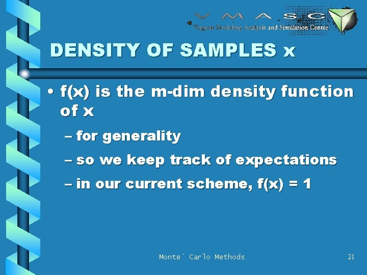
DENSITY OF SAMPLES x • f(x) is the m-dim density function of x – for generality – so we keep track of expectations – in our current scheme, f(x) = 1 Monte` Carlo Methods 21

LAMBDA AYE Monte` Carlo Methods 22

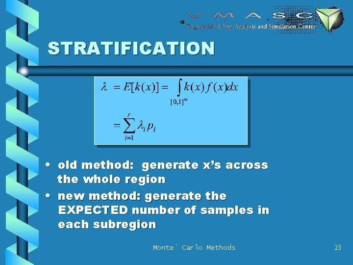
STRATIFICATION • old method: generate x’s across the whole region • new method: generate the EXPECTED number of samples in each subregion Monte` Carlo Methods 23

• let Xj be the jth sample in the old method capitols indicate random samples! Monte` Carlo Methods 24

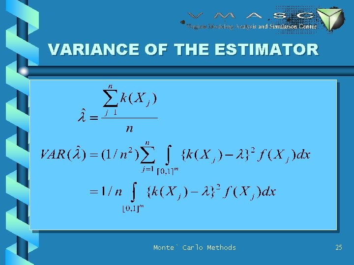
VARIANCE OF THE ESTIMATOR Monte` Carlo Methods 25

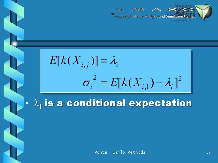
STRATIFICATION • Generate n 1, n 2, . . . , nr samples from A 1, A 2, . . . , Ar – on purpose • ni = npi • ni sum to n • Xi, j is jth sample from Ai Monte` Carlo Methods 26

• li is a conditional expectation Monte` Carlo Methods 27

Monte` Carlo Methods 28

Monte` Carlo Methods 29

Monte` Carlo Methods 30

HOW THAT LAST BIT WORKED Monte` Carlo Methods 31

. . . AND SO. . . • Stratification reduces the variance of the estimator • A random quantity (the samples pulled from Ai) is replaced by its expectation • This only works because of all of the SUMMATION and no other complicated functions Monte` Carlo Methods 32

FOR THE SPHERE PROBLEM • 500 samples – Divide evenly in 64 cubes • 4 X 4 • 7 or 8 samples in each cube – 64 separate l’s – Add together • How did we know to start with 500? Monte` Carlo Methods 33

Discussion of applications. . . Monte` Carlo Methods 34