Montague meets Markov Combining Logical and Distributional Semantics

Montague meets Markov: Combining Logical and Distributional Semantics Raymond J. Mooney Katrin Erk Islam Beltagy University of Texas at Austin 1

Logical AI Paradigm • Represents knowledge and data in a binary symbolic logic such as FOPC. + Rich representation that handles arbitrary sets of objects, with properties, relations, quantifiers, etc. Unable to handle uncertain knowledge and probabilistic reasoning.

Probabilistic AI Paradigm • Represents knowledge and data as a fixed set of random variables with a joint probability distribution. + Handles uncertain knowledge and probabilistic reasoning. Unable to handle arbitrary sets of objects, with properties, relations, quantifiers, etc.

Statistical Relational Learning (SRL) • SRL methods attempt to integrate methods from predicate logic (or relational databases) and probabilistic graphical models to handle structured, multi-relational data.

SRL Approaches (A Taste of the “Alphabet Soup”) • Stochastic Logic Programs (SLPs) (Muggleton, 1996) • Probabilistic Relational Models (PRMs) (Koller, 1999) • Bayesian Logic Programs (BLPs) (Kersting & De Raedt, 2001) • Markov Logic Networks (MLNs) (Richardson & Domingos, 2006) • Probabilistic Soft Logic (PSL) (Kimmig et al. , 2012) • 5

SRL Methods Based on Probabilistic Graphical Models • BLPs use definite-clause logic (Prolog programs) to define abstract templates for large, complex Bayesian networks (i. e. directed graphical models). • MLNs use full first order logic to define abstract templates for large, complex Markov networks (i. e. undirected graphical models). • PSL uses logical rules to define templates for Markov nets with real-valued propositions to support efficient inference. • Mc. Callum’s FACTORIE uses an object-oriented programming language to define large, complex factor graphs. • Goodman & Tanenbaum’s CHURCH uses a functional programming language to define, large complex generative models. 6

Markov Logic Networks [Richardson & Domingos, 2006] Set of weighted clauses in first-order predicate logic. Larger weight indicates stronger belief that the clause should hold. MLNs are templates for constructing Markov networks for a given set of constants MLN Example: Friends & Smokers 7

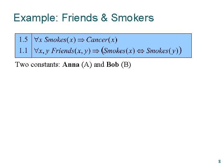
Example: Friends & Smokers Two constants: Anna (A) and Bob (B) 8

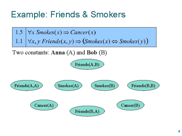
Example: Friends & Smokers Two constants: Anna (A) and Bob (B) Friends(A, A) Smokes(B) Cancer(A) Friends(B, B) Cancer(B) Friends(B, A) 9

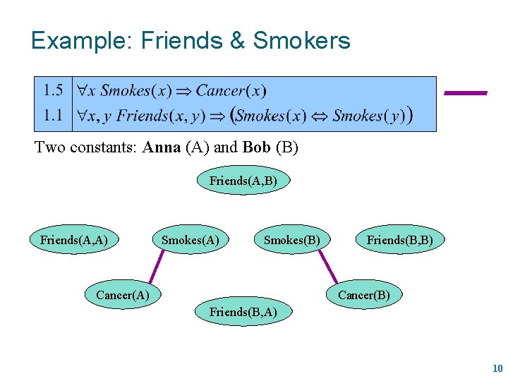
Example: Friends & Smokers Two constants: Anna (A) and Bob (B) Friends(A, A) Smokes(B) Cancer(A) Friends(B, B) Cancer(B) Friends(B, A) 10

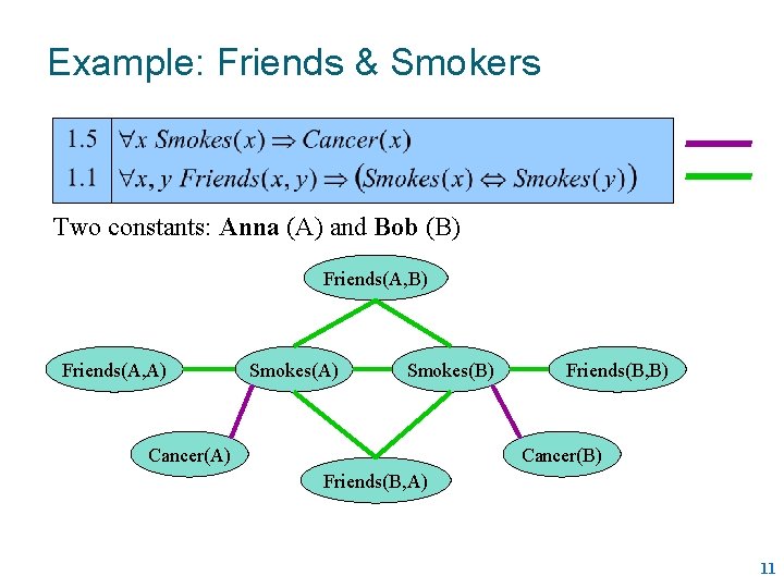
Example: Friends & Smokers Two constants: Anna (A) and Bob (B) Friends(A, A) Smokes(B) Cancer(A) Friends(B, B) Cancer(B) Friends(B, A) 11

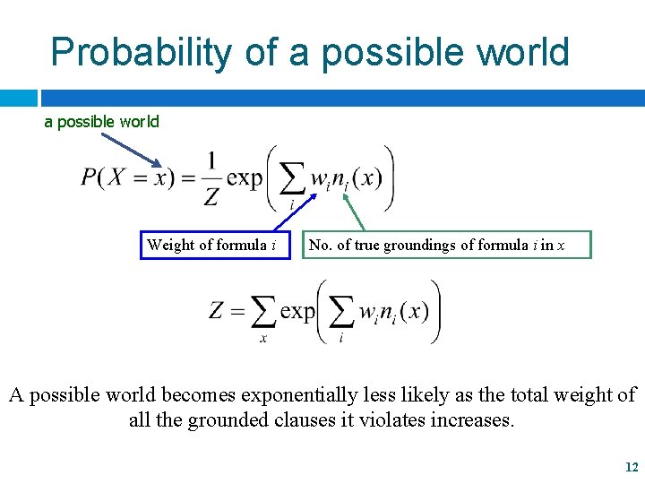
Probability of a possible world Weight of formula i No. of true groundings of formula i in x A possible world becomes exponentially less likely as the total weight of all the grounded clauses it violates increases. 12

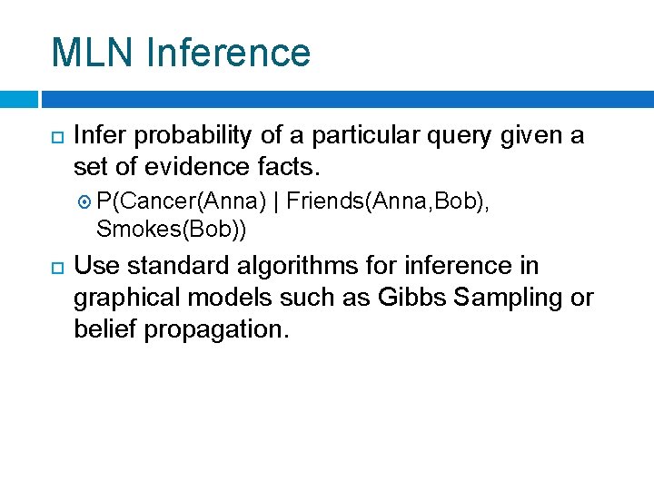
MLN Inference Infer probability of a particular query given a set of evidence facts. P(Cancer(Anna) | Friends(Anna, Bob), Smokes(Bob)) Use standard algorithms for inference in graphical models such as Gibbs Sampling or belief propagation.

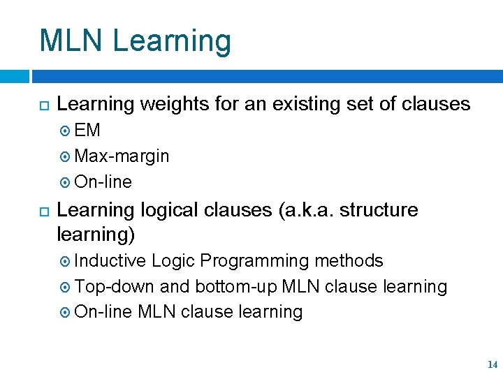
MLN Learning weights for an existing set of clauses EM Max-margin On-line Learning logical clauses (a. k. a. structure learning) Inductive Logic Programming methods Top-down and bottom-up MLN clause learning On-line MLN clause learning 14

Strengths of MLNs • Fully subsumes first-order predicate logic – Just give weight to all clauses • Fully subsumes probabilistic graphical models. – Can represent any joint distribution over an arbitrary set of discrete random variables. • Can utilize prior knowledge in both symbolic and probabilistic forms. • Large existing base of open-source software (Alchemy) 15

Weaknesses of MLNs • Inherits computational intractability of general methods for both logical and probabilistic inference and learning. – Inference in FOPC is semi-decidable – Inference in general graphical models is P-space complete • Just producing the “ground” Markov Net can produce a combinatorial explosion. – Current “lifted” inference methods do not help reasoning with many kinds of nested quantifiers. 16

PSL: Probabilistic Soft Logic [Kimmig & Bach & Broecheler & Huang & Getoor, NIPS 2012] ● ● ● Probabilistic logic framework designed with efficient inference in mind. Input: set of weighted First Order Logic rules and a set of evidence, just as in BLP or MLN MPE inference is a linear-programming problem that can efficiently draw probabilistic conclusions. 17

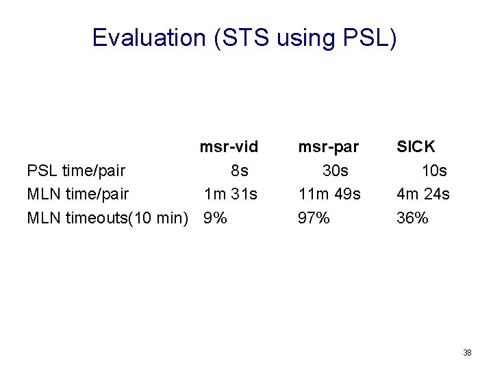
PSL vs. MLN PSL ● ● Atoms have continuous truth values in the interval [0, 1]. Inference finds truth value of all atoms that best satisfy the rules and evidence. MPE inference: Most Probable Explanation. Linear optimization problem. ● ● Atoms have boolean truth values {0, 1}. Inference finds probability of atoms given the rules and evidence. Calculates conditional probability of a query atom given evidence. Combinatorial counting problem. 18

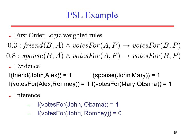
PSL Example ● First Order Logic weighted rules ● Evidence I(friend(John, Alex)) = 1 I(spouse(John, Mary)) = 1 I(votes. For(Alex, Romney)) = 1 I(votes. For(Mary, Obama)) = 1 ● Inference – – I(votes. For(John, Obama)) = 1 I(votes. For(John, Romney)) = 0 19

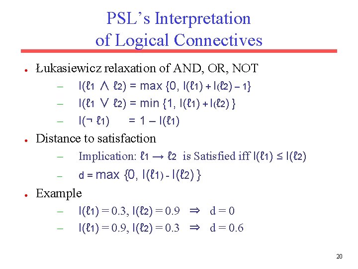
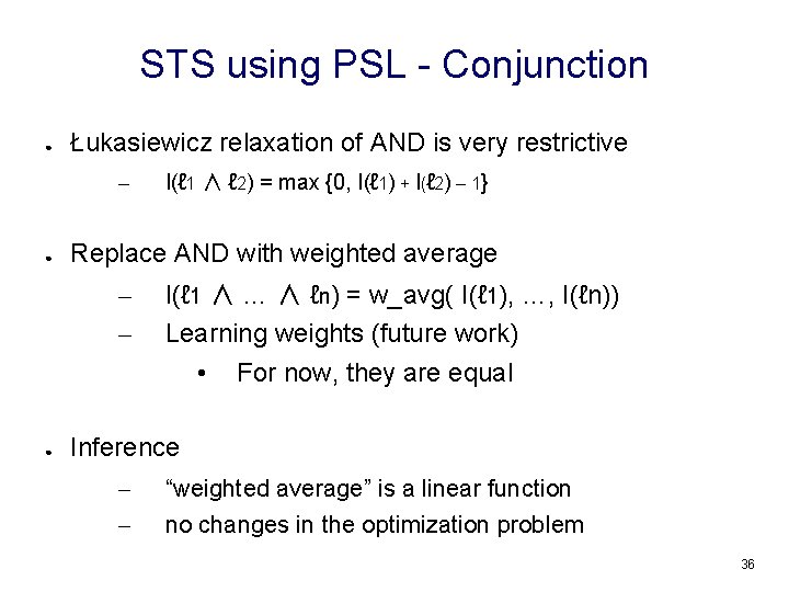
PSL’s Interpretation of Logical Connectives ● Łukasiewicz relaxation of AND, OR, NOT – – – ● ● I(ℓ 1 ∧ ℓ 2) = max {0, I(ℓ 1) + I(ℓ 2) – 1} I(ℓ 1 ∨ ℓ 2) = min {1, I(ℓ 1) + I(ℓ 2) } I(¬ ℓ 1) = 1 – I(ℓ 1) Distance to satisfaction – Implication: ℓ 1 → ℓ 2 is Satisfied iff I(ℓ 1) ≤ I(ℓ 2) – d = max {0, I(ℓ 1) - I(ℓ 2) } Example – – I(ℓ 1) = 0. 3, I(ℓ 2) = 0. 9 ⇒ d = 0 I(ℓ 1) = 0. 9, I(ℓ 2) = 0. 3 ⇒ d = 0. 6 20

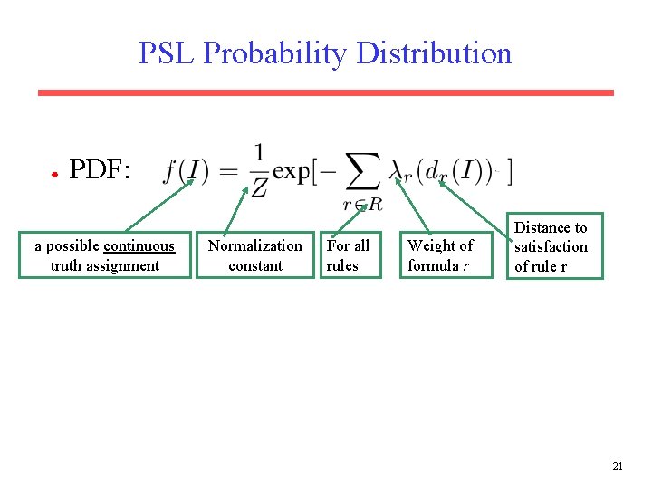
PSL Probability Distribution ● PDF: a possible continuous truth assignment Normalization constant For all rules Weight of formula r Distance to satisfaction of rule r 21

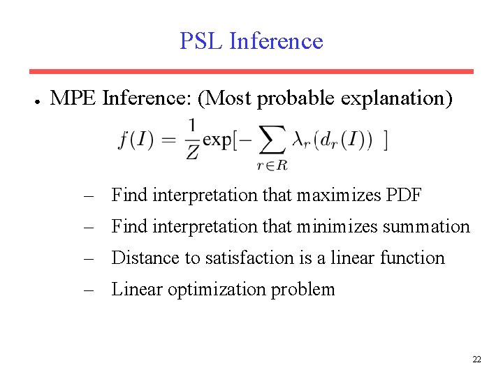
PSL Inference ● MPE Inference: (Most probable explanation) – Find interpretation that maximizes PDF – Find interpretation that minimizes summation – Distance to satisfaction is a linear function – Linear optimization problem 22

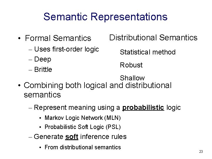
Semantic Representations • Formal Semantics – Uses first-order logic – Deep – Brittle Distributional Semantics Statistical method Robust Shallow • Combining both logical and distributional semantics – Represent meaning using a probabilistic logic • Markov Logic Network (MLN) • Probabilistic Soft Logic (PSL) – Generate soft inference rules • From distributional semantics 23

System Architecture [Garrette et al. 2011, 2012; Beltagy et al. , 2013] Sent 1 Sent 2 BOXER LF 1 LF 2 Dist. Rule Constructor Vector Space • BOXER [Bos, et al. 2004]: maps sentences to logical form Rule Base MLN/PSL Inference result • Distributional Rule constructor: generates relevant soft inference rules based on distributional similarity • MLN/PSL: probabilistic inference • Result: degree of entailment or semantic similarity score (depending on the task) 24

Markov Logic Networks [Richardson & Domingos, 2006] • Two constants: Anna (A) and Bob (B) Friends(A, A) Smokes(B) Cancer(A) Friends(B, B) Cancer(B) Friends(B, A) • P(Cancer(Anna) | Friends(Anna, Bob), Smokes(Bob)) 25

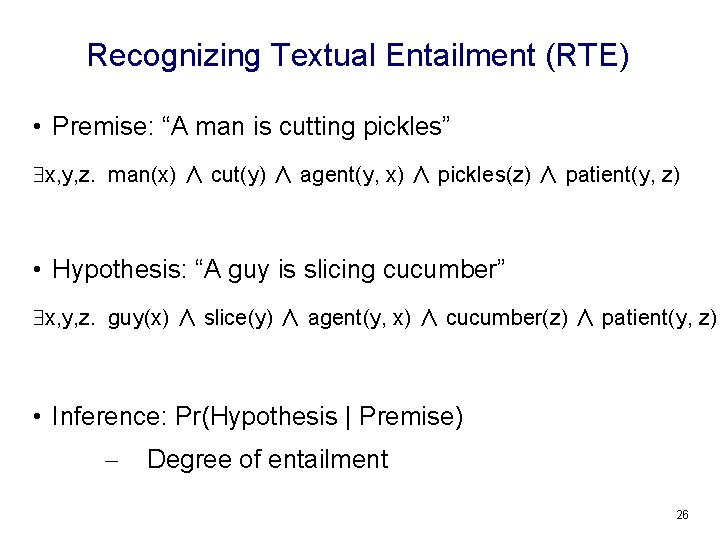
Recognizing Textual Entailment (RTE) • Premise: “A man is cutting pickles” x, y, z. man(x) ∧ cut(y) ∧ agent(y, x) ∧ pickles(z) ∧ patient(y, z) • Hypothesis: “A guy is slicing cucumber” x, y, z. guy(x) ∧ slice(y) ∧ agent(y, x) ∧ cucumber(z) ∧ patient(y, z) • Inference: Pr(Hypothesis | Premise) – Degree of entailment 26

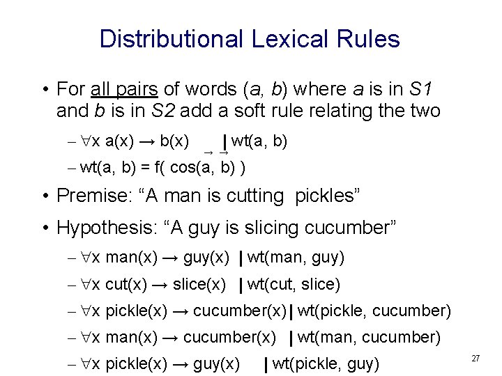
Distributional Lexical Rules • For all pairs of words (a, b) where a is in S 1 and b is in S 2 add a soft rule relating the two – x a(x) → b(x) | wt(a, b) → → – wt(a, b) = f( cos(a, b) ) • Premise: “A man is cutting pickles” • Hypothesis: “A guy is slicing cucumber” – x man(x) → guy(x) | wt(man, guy) – x cut(x) → slice(x) | wt(cut, slice) – x pickle(x) → cucumber(x) | wt(pickle, cucumber) – x man(x) → cucumber(x) | wt(man, cucumber) – x pickle(x) → guy(x) | wt(pickle, guy) 27

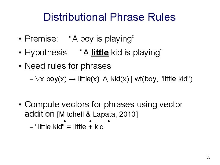
Distributional Phrase Rules • Premise: “A boy is playing” • Hypothesis: “A little kid is playing” • Need rules for phrases – x boy(x) → little(x) ∧ kid(x) | wt(boy, "little kid") • Compute vectors for phrases using vector addition [Mitchell & Lapata, 2010] – "little kid" = little + kid 28

Paraphrase Rules [by: Cuong Chau] • Generate inference rules from pre-compiled paraphrase collections like Berant et al. [2012] • e. g, “X solves Y” => “X finds a solution to Y ” | w 29

Evaluation (RTE using MLNs) • Dataset • RTE-1, RTE-2, RTE-3 • Each dataset is 800 training pairs and 800 testing pairs • Use multiple parses to reduce impact of misparses 30

Evaluation (RTE using MLNs) [by: Cuong Chau] Logic-only baseline KB is wordnet RTE-1 RTE-2 RTE-3 Bos & Markert[2005] 0. 52 – – MLN 0. 57 0. 58 0. 55 MLN-multi-parse 0. 56 0. 58 0. 57 MLN-paraphrases 0. 60 31

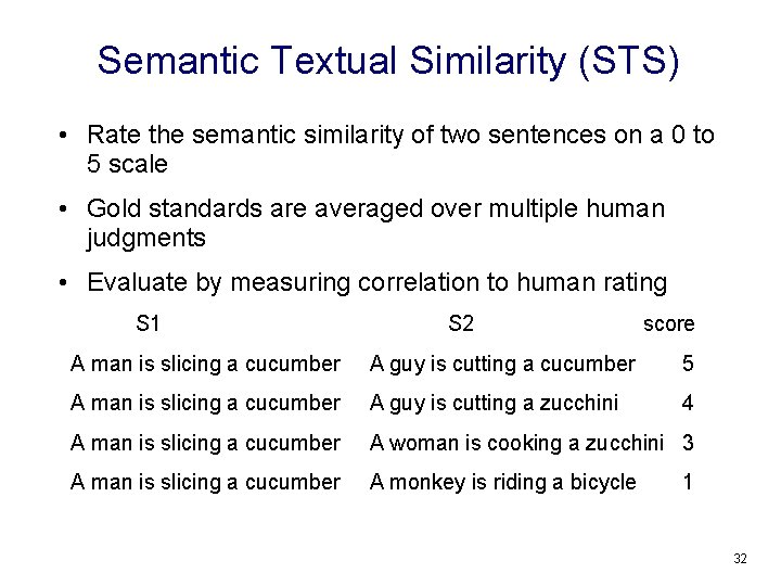
Semantic Textual Similarity (STS) • Rate the semantic similarity of two sentences on a 0 to 5 scale • Gold standards are averaged over multiple human judgments • Evaluate by measuring correlation to human rating S 1 S 2 score A man is slicing a cucumber A guy is cutting a cucumber 5 A man is slicing a cucumber A guy is cutting a zucchini 4 A man is slicing a cucumber A woman is cooking a zucchini 3 A man is slicing a cucumber A monkey is riding a bicycle 1 32

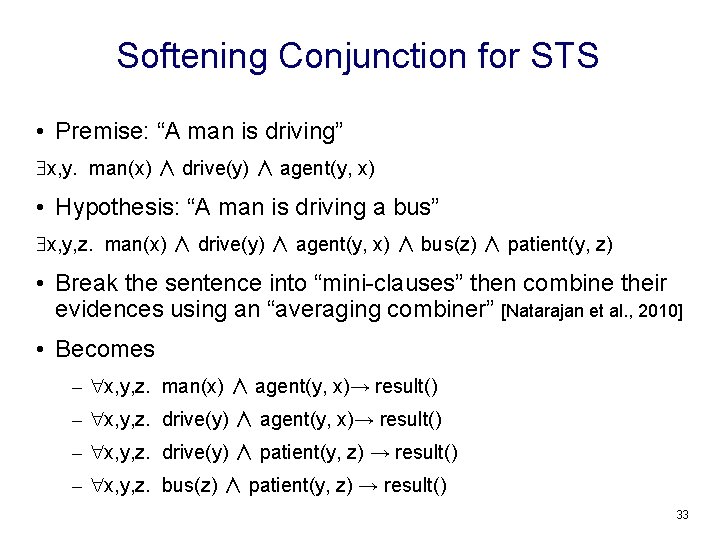
Softening Conjunction for STS • Premise: “A man is driving” x, y. man(x) ∧ drive(y) ∧ agent(y, x) • Hypothesis: “A man is driving a bus” x, y, z. man(x) ∧ drive(y) ∧ agent(y, x) ∧ bus(z) ∧ patient(y, z) • Break the sentence into “mini-clauses” then combine their evidences using an “averaging combiner” [Natarajan et al. , 2010] • Becomes – x, y, z. man(x) ∧ agent(y, x)→ result() – x, y, z. drive(y) ∧ patient(y, z) → result() – x, y, z. bus(z) ∧ patient(y, z) → result() 33

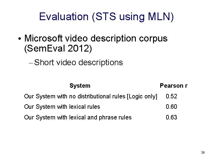
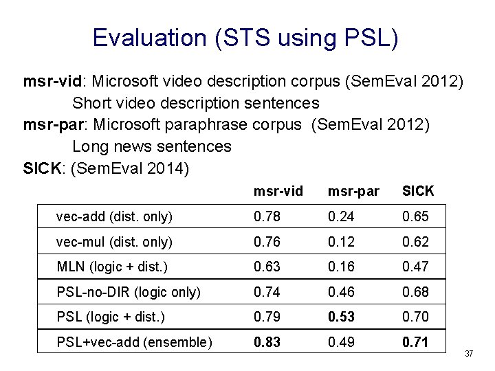
Evaluation (STS using MLN) • Microsoft video description corpus (Sem. Eval 2012) – Short video descriptions System Pearson r Our System with no distributional rules [Logic only] 0. 52 Our System with lexical rules 0. 60 Our System with lexical and phrase rules 0. 63 34

PSL: Probabilistic Soft Logic [Kimmig & Bach & Broecheler & Huang & Getoor, NIPS 2012] ● ● ● MLN's inference is very slow PSL is a probabilistic logic framework designed with efficient inference in mind Inference is a linear program 35

STS using PSL - Conjunction ● Łukasiewicz relaxation of AND is very restrictive – ● Replace AND with weighted average – – ● I(ℓ 1 ∧ ℓ 2) = max {0, I(ℓ 1) + I(ℓ 2) – 1} I(ℓ 1 ∧ … ∧ ℓn) = w_avg( I(ℓ 1), …, I(ℓn)) Learning weights (future work) • For now, they are equal Inference – – “weighted average” is a linear function no changes in the optimization problem 36

Evaluation (STS using PSL) msr-vid: Microsoft video description corpus (Sem. Eval 2012) Short video description sentences msr-par: Microsoft paraphrase corpus (Sem. Eval 2012) Long news sentences SICK: (Sem. Eval 2014) msr-vid msr-par SICK vec-add (dist. only) 0. 78 0. 24 0. 65 vec-mul (dist. only) 0. 76 0. 12 0. 62 MLN (logic + dist. ) 0. 63 0. 16 0. 47 PSL-no-DIR (logic only) 0. 74 0. 46 0. 68 PSL (logic + dist. ) 0. 79 0. 53 0. 70 PSL+vec-add (ensemble) 0. 83 0. 49 0. 71 37

Evaluation (STS using PSL) msr-vid PSL time/pair 8 s MLN time/pair 1 m 31 s MLN timeouts(10 min) 9% msr-par 30 s 11 m 49 s 97% SICK 10 s 4 m 24 s 36% 38