Monopolistic Competition and Basic Oligopoly Models Monopolistic Competition
Monopolistic Competition and Basic Oligopoly Models
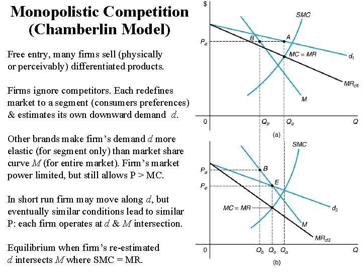
Monopolistic Competition (Chamberlin Model) Free entry, many firms sell (physically or perceivably) differentiated products. Firms ignore competitors. Each redefines market to a segment (consumers preferences) & estimates its own downward demand d. Other brands make firm’s demand d more elastic (for segment only) than market share curve M (for entire market). Firm’s market power limited, but still allows P > MC. In short run firm may move along d, but eventually similar conditions lead to similar P: each firm operates at d & M intersection. Equilibrium when firm’s re-estimated d intersects M where SMC = MR.
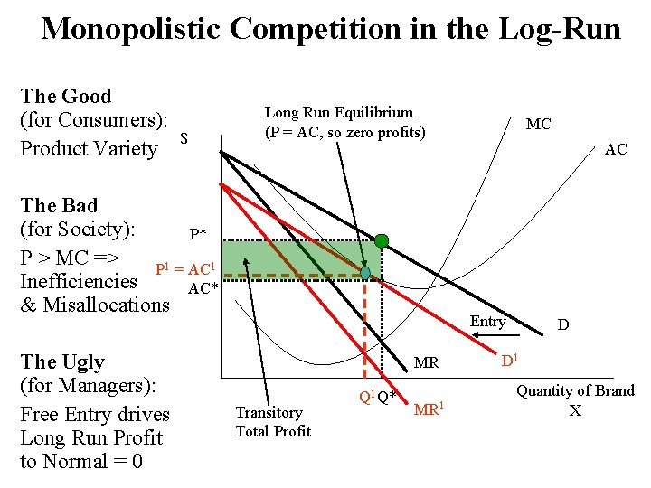
Monopolistic Competition in the Log-Run The Good (for Consumers): Product Variety $ Long Run Equilibrium (P = AC, so zero profits) The Bad (for Society): P* P > MC => P 1 = AC 1 Inefficiencies AC* & Misallocations The Ugly (for Managers): Free Entry drives Long Run Profit to Normal = 0 MC AC Entry MR Transitory Total Profit Q 1 Q* MR 1 D D 1 Quantity of Brand X
Strategies to Avoid (or Delay) the Zero Profit Outcome • Change; don’t let the long-run set in. • Be the first to introduce new brands or to improve existing products and services. • Seek out sustainable niches. • Create barriers to entry. • Increase the time it takes others to clone your brand with “trade secrets” and “strategic plans”.
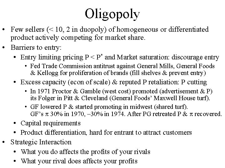
Oligopoly • Few sellers (< 10, 2 in duopoly) of homogeneous or differentiated product actively competing for market share. • Barriers to entry: • Entry limiting pricing P < P* and Market saturation: discourage entry • Fed Trade Commission antitrust against General Mills, General Foods & Kellogg for proliferation of brands (fill shelves & prevent entry) • Excess capacity (econ of scale) & reputed P retaliation: P cutting • In 1971 Proctor & Gamble (west cost) promoted (advertisement & P) its Folger in Pitt & Cleveland (General Foods’ Maxwell House turf). • GF lowered P & started promoting in midwest (shared turf). GF’s 30% in 1970, – 30% in 1974. After PG retreated P & recovered. • Capital requirements • Product differentiation, hard for entrant to attract customers • Strategic Interaction • What you do affects the profits of your rivals • What your rival does affects your profits
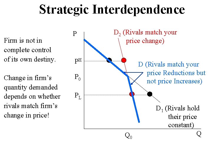
Strategic Interdependence Firm is not in complete control of its own destiny. Change in firm’s quantity demanded depends on whether rivals match firm’s change in price! P D 2 (Rivals match your price change) PH D (Rivals match your price Reductions but not price Increases) P 0 PL Q 0 D 1 (Rivals hold their price constant) Q
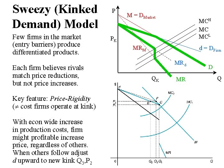
Sweezy (Kinked Demand) Model Few firms in the market (entry barriers) produce differentiated products. Each firm believes rivals match price reductions, but not price increases. Key feature: Price-Rigidity ( cost firms operate at kink) With econ wide increase in production costs, firm might profitable increase price, regardless of others. When others follow adjust d upward to new kink Q 3, P 2 P M = DMarket MCH MC MCL PK MRM d = DFirm MRd QK MR D Q
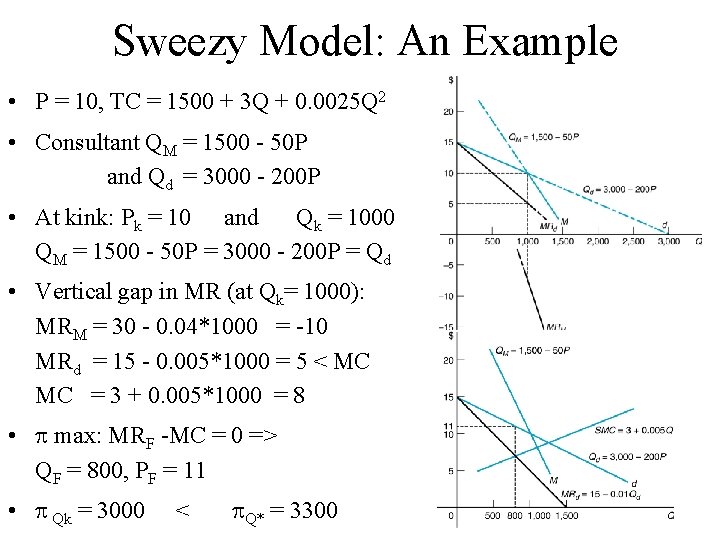
Sweezy Model: An Example • P = 10, TC = 1500 + 3 Q + 0. 0025 Q 2 • Consultant QM = 1500 - 50 P and Qd = 3000 - 200 P • At kink: Pk = 10 and Qk = 1000 QM = 1500 - 50 P = 3000 - 200 P = Qd • Vertical gap in MR (at Qk= 1000): MRM = 30 - 0. 04*1000 = -10 MRd = 15 - 0. 005*1000 = 5 < MC MC = 3 + 0. 005*1000 = 8 • max: MRF -MC = 0 => QF = 800, PF = 11 • Qk = 3000 < Q* = 3300
Cournot Duopoly • Two firms produce homogenous product in an industry with barriers to entry • Firms maximize profit by setting output, as opposed to price • Each firm wrongly believes their rival will hold output constant if it changes its own output • Firm’s reaction (or best-response) function: profit maximizing amount of output for each quantity of output produced by rival
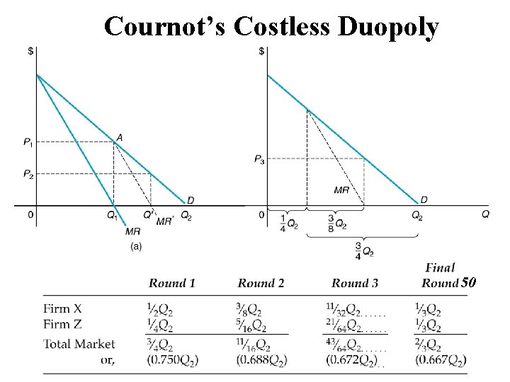
Cournot’s Costless Duopoly 50
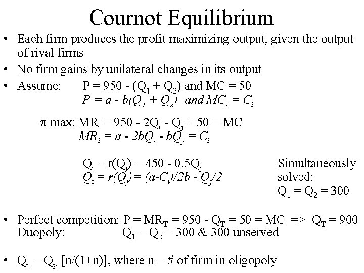
Cournot Equilibrium • Each firm produces the profit maximizing output, given the output of rival firms • No firm gains by unilateral changes in its output • Assume: P = 950 - (Q 1 + Q 2) and MC = 50 P = a - b(Q 1 + Q 2) and MCi = Ci max: MRi = 950 - 2 Qi - Qj = 50 = MC MRi = a - 2 b. Qi - b. Qj = Ci Qi = r(Qj) = 450 - 0. 5 Qj Qi = r(Qj)= (a-Ci)/2 b - Qj/2 Simultaneously solved: Q 1 = Q 2 = 300 • Perfect competition: P = MRT = 950 - QT = 50 = MC => QT = 900 Duopoly: Q 1 = Q 2 = 300 & 300 unserved • Qn = Qpc[n/(1+n)], where n = # of firm in oligopoly
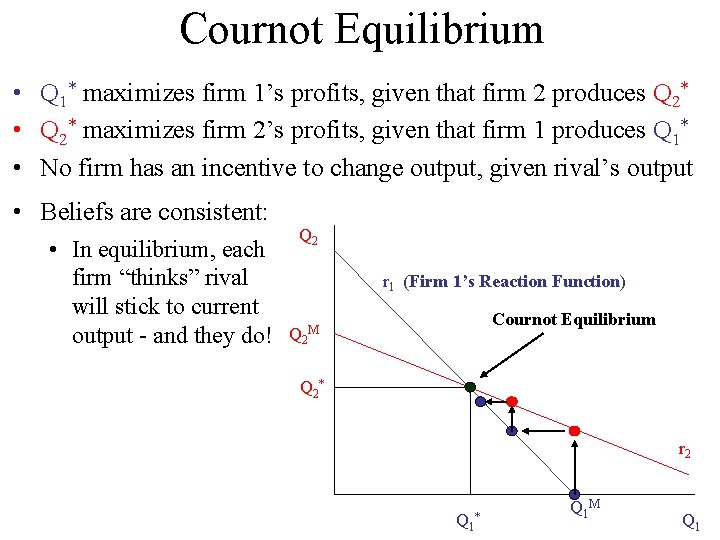
Cournot Equilibrium • Q 1* maximizes firm 1’s profits, given that firm 2 produces Q 2* • Q 2* maximizes firm 2’s profits, given that firm 1 produces Q 1* • No firm has an incentive to change output, given rival’s output • Beliefs are consistent: • In equilibrium, each firm “thinks” rival will stick to current output - and they do! Q 2 r 1 (Firm 1’s Reaction Function) Cournot Equilibrium Q 2 M Q 2 * r 2 Q 1 * Q 1 M Q 1
Stackelberg Model • Few firms produce differentiated or homogeneous products in industry with barriers to entry • Firm leader commits to an output before followers • Remaining firms, followers, profit maximizing outputs, given the leader’s output. • Commitment and first-mover advantage can enhance profits in strategic environments • Leader produces more than in Cournot equilibrium (Larger market share, higher profits) • Follower produces less than in Cournot equilibrium (Smaller market share, lower profits)
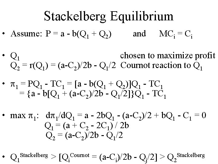
Stackelberg Equilibrium • Assume: P = a - b(Q 1 + Q 2) and MCi = Ci • Q 1 chosen to maximize profit Q 2 = r(Q 1) = (a-C 2)/2 b - Q 1/2 Cournot reaction to Q 1 • 1 = PQ 1 - TC 1 = [a - b(Q 1 + Q 2)]Q 1 - TC 1 = {a - b[Q 1 + (a-C 2)/2 b - Q 1/2]}Q 1 - TC 1 • max 1: d 1/d. Q 1 = a - 2 b. Q 1 - (a-C 2)/2 + b. Q 1 - C 1 = 0 Q 1 = (a + C 2 - 2 C 1) / 2 b Q 2 = (a-C 2)/2 b - Q 1/2 • Q 1 Stackelberg > [Qi. Cournot = (a-Ci)/2 b - Qj/2] > Q 2 Stackelberg
Bertrand Edgeworth Duopoly • Two firms produce identical products at constant MC, in an industry with barriers to entry • Each firm independently sets its profit maximizing price • Consumers have perfect knowledge & no transaction costs • Suppose MC < P 1 < P 2 • Firm 1 earns (P 1 - MC) per unit and firm 2 earns nothing • Firm 2 undercuts firm 1’s price to capture the entire market • Firm 1 then undercuts firm 2’s price • Undercutting continues until equilibrium: P 1 = P 2 = MC • Perfect competition profit maximizing solution P = MC possible with few firms and severe price competition • If duopolists have limited capacity relative to the Bertrand equilibrium, Edgeworth argued that price will not be stable
Chamberlin Duopoly • Chamberlin applied results from his analysis of monopolistic competition on oligopoly • Cournot, Bertrand Edgeworth models assume that competitors are extremely naïve • Chamberlin argued that oligopolists would recognize their mutual or strategic interdependence and engage in tacit or informal collusion: independently choose monopoly price and split profits • Managers signal to competitors their desire not to engage in destructive price war by setting price • Agreements are not necessary because firms realize any other strategy is less profitable • Formal Collusive agreements are illegal, although U. S. firms have been permitted to agree on export pricing
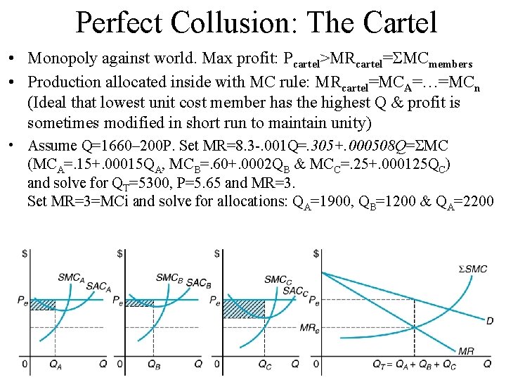
Perfect Collusion: The Cartel • Monopoly against world. Max profit: Pcartel>MRcartel= MCmembers • Production allocated inside with MC rule: MRcartel=MCA=…=MCn (Ideal that lowest unit cost member has the highest Q & profit is sometimes modified in short run to maintain unity) • Assume Q=1660– 200 P. Set MR=8. 3 -. 001 Q=. 305+. 000508 Q= MC (MCA=. 15+. 00015 QA, MCB=. 60+. 0002 QB & MCC=. 25+. 000125 QC) and solve for QT=5300, P=5. 65 and MR=3. Set MR=3=MCi and solve for allocations: QA=1900, QB=1200 & QA=2200
Contestable Markets • Few sellers but free entry: Oligopoly will price at a perfect competition level & have only normal = 0 • Key Assumptions • Producers have access to same technology • Consumers respond quickly to price changes • Existing firms cannot respond quickly to entry by lowering price • Absence of sunk costs • Key Implications • Threat of entry disciplines firms already in the market • Incumbents have no market power, even if there is only a single incumbent (a monopolist)
Summary • Different oligopoly scenarios lead to different optimal strategies and different outcomes • Your optimal price and output depends on … • Beliefs about the reactions of rivals • Your choice variable (P or Q) and the nature of the product market (differentiated or homogeneous products) • Your ability to commit
- Slides: 19