Monitoring Active Portfolios The CUSUM Approach Thomas K

Monitoring Active Portfolios: The CUSUM Approach Thomas K. Philips Chief Investment Officer Paradigm Asset Management (joint work with D. Stein and E. Yashchin)

Agenda § Portfolio monitoring: problem formulation & description § Sequential testing and process control § The Cusum scheme – Economic intuition, simplified theory & implementation § Issues that arise in practice – Optimality and robustness – Causality 2

The Investor’s / CIO’s Problem § Invested in / responsible for many active products – Fallout of the asset allocation / manager selection / sales / reseach / product development process § Lots of data coming in from portfolio managers – Returns, portfolio holdings, sector allocations, risk profiles, transactions etc. § Not clear which portfolios merit extra attention – Investor / CIO will ideally focus on products that might be in trouble 3

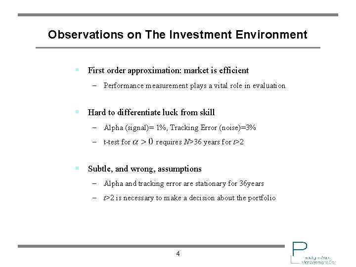
Observations on The Investment Environment § First order approximation: market is efficient – Performance measurement plays a vital role in evaluation § Hard to differentiate luck from skill – Alpha (signal)= 1%, Tracking Error (noise)=3% – t-test for requires N>36 years for t>2 § Subtle, and wrong, assumptions – Alpha and tracking error are stationary for 36 years – t>2 is necessary to make a decision about the portfolio 4

Performance Measurement in Practice § Performance measurement is rooted in classical statistics § Measure benchmark relative performance over fixed & rolling intervals – 3 to 5 years is common – Extrapolate trends in rolling benchmark or peer group relative performance – Focus attention on the underperforming products § Cannot identify regime changes or shifts in performance – t-stats are too low to be meaningful – Not clear if attention is focused on the right products at the right time 5

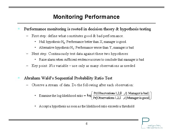
Monitoring Performance § Performance monitoring is rooted in decision theory & hypothesis testing – First step: define what constitutes good & bad performance. • Null hypothesis H 0: Performance better than X, manager is good. • Alternative hypothesis H 1: Performance worse than Y, manager is bad – Next step: Continuously test data against these two hypotheses • Raise alarm when sufficient evidence accrues to conclude that manager is bad – Key point: N is variable – use only as many observations as needed § Abraham Wald’s Sequential Probability Ratio Test – Observe a stream of data. Do the following after each observation: • Examine the log-likelihood ratio = • Accept a hypothesis as soon as the likelihood ratio exceeds a threshold 6

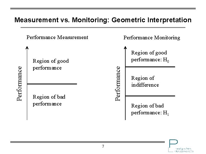
Measurement vs. Monitoring: Geometric Interpretation Performance Monitoring Region of good performance: H 0 Region of good performance Performance Measurement Region of bad performance Region of indifference Region of bad performance: H 1 7

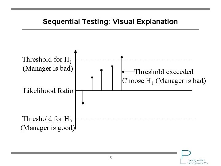
Sequential Testing: Visual Explanation Threshold for H 1 (Manager is bad) Threshold exceeded Choose H 1 (Manager is bad) Likelihood Ratio Threshold for H 0 (Manager is good) 8

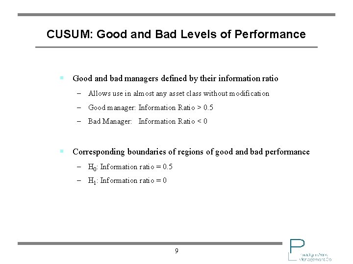
CUSUM: Good and Bad Levels of Performance § Good and bad managers defined by their information ratio – Allows use in almost any asset class without modification – Good manager: Information Ratio > 0. 5 – Bad Manager: Information Ratio < 0 § Corresponding boundaries of regions of good and bad performance – H 0: Information ratio = 0. 5 – H 1: Information ratio = 0 9

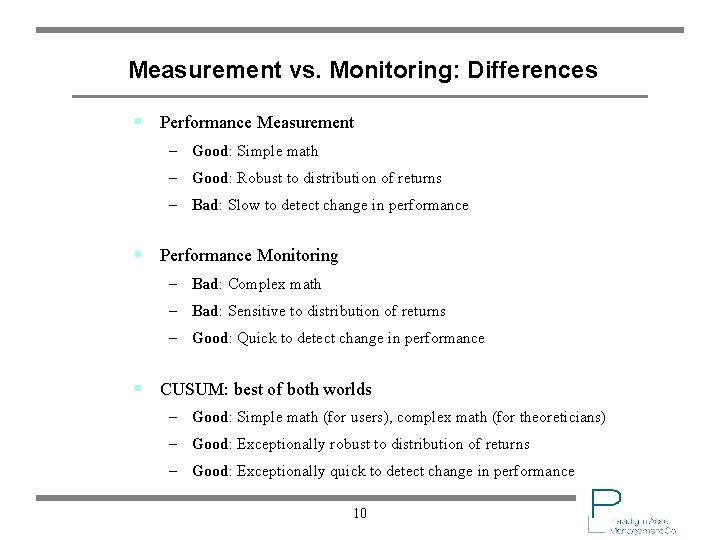
Measurement vs. Monitoring: Differences § Performance Measurement – Good: Simple math – Good: Robust to distribution of returns – Bad: Slow to detect change in performance § Performance Monitoring – Bad: Complex math – Bad: Sensitive to distribution of returns – Good: Quick to detect change in performance § CUSUM: best of both worlds – Good: Simple math (for users), complex math (for theoreticians) – Good: Exceptionally robust to distribution of returns – Good: Exceptionally quick to detect change in performance 10

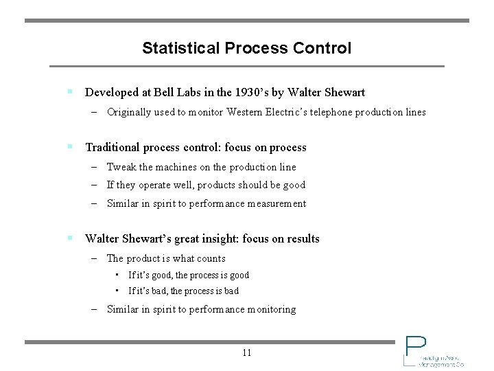
Statistical Process Control § Developed at Bell Labs in the 1930’s by Walter Shewart – Originally used to monitor Western Electric’s telephone production lines § Traditional process control: focus on process – Tweak the machines on the production line – If they operate well, products should be good – Similar in spirit to performance measurement § Walter Shewart’s great insight: focus on results – The product is what counts • If it’s good, the process is good • If it’s bad, the process is bad – Similar in spirit to performance monitoring 11

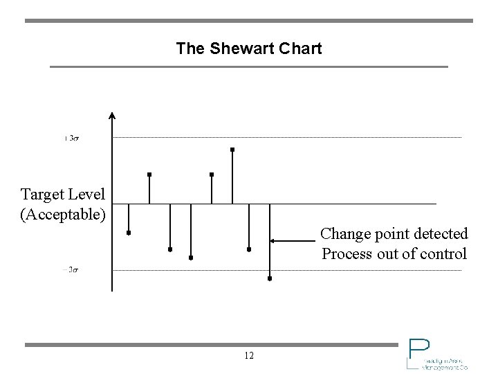
The Shewart Chart Target Level (Acceptable) Change point detected Process out of control 12

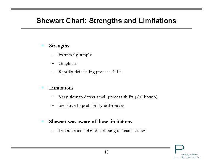
Shewart Chart: Strengths and Limitations § Strengths – Extremely simple – Graphical – Rapidly detects big process shifts § Limitations – Very slow to detect small process shifts (-10 bp/mo) – Sensitive to probability distribution § Shewart was aware of these limitations – Did not succeed in developing a clean solution 13

The CUSUM Technique § Created by E. S. Page in 1954 § Addresses the limitations of the Shewart chart – Reliably detects small process shifts – Insensitive to probability distribution § Provably optimal: detects process shifts faster than any other method – Proof (Moustakides) is very hard. Uses optional stopping theorem. – Extremely robust, good under almost any definition of optimality • Much better than exponentially weighted moving average 14

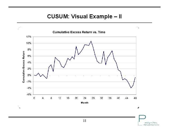
Page’s Great Insight § Plot the cumulative arithmetic sum of residuals (e. g. excess returns) – Cumulating filters noise, strengthens signal • Positive process mean Positive slope • Negative process mean Negative slope • 0 process mean 0 slope (flat) § Changes in slope are easily detected, both visually and mathematically – Cusum is a very clever variant of the Sequential Probability Ratio Test – Raise an alarm if the cumulative sum becomes large and negative § Works about as well as the Shewart chart for large process shifts – Works much faster for small process shifts – Particularly well suited to money management 15

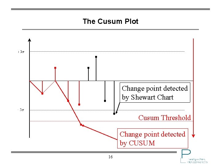
The Cusum Plot Change point detected by Shewart Chart Cusum Threshold Change point detected by CUSUM 16

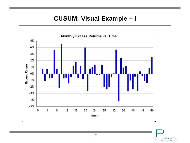
CUSUM: Visual Example – I 17

CUSUM: Visual Example – II 18

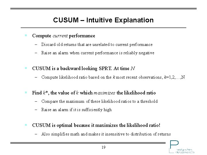
CUSUM – Intuitive Explanation § Compute current performance – Discard old returns that are unrelated to current performance – Raise an alarm when current performance is reliably negative § CUSUM is a backward looking SPRT. At time N – Compute likelihood ratio based on the k most recent observations, k=1, 2, …, N § Find k*, the value of k which maximizes the likelihood ratio – Compare the maximum of these likelihood ratios to a threshold – Raise an alarm if it is sufficiently high § CUSUM is optimal because it maximizes the likelihood ratio! – Also simplifies math and makes it insensitive to distribution of returns 19

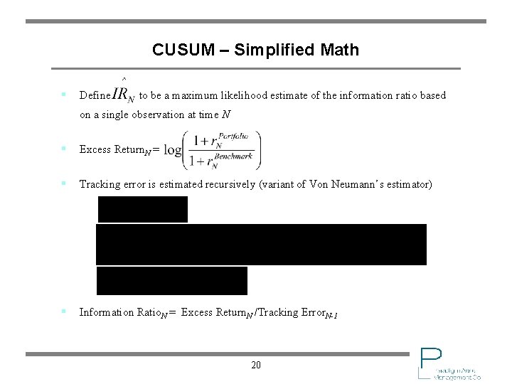
CUSUM – Simplified Math § Define to be a maximum likelihood estimate of the information ratio based on a single observation at time N § Excess Return. N = § Tracking error is estimated recursively (variant of Von Neumann’s estimator) § Information Ratio. N = Excess Return. N /Tracking Error. N-1 20

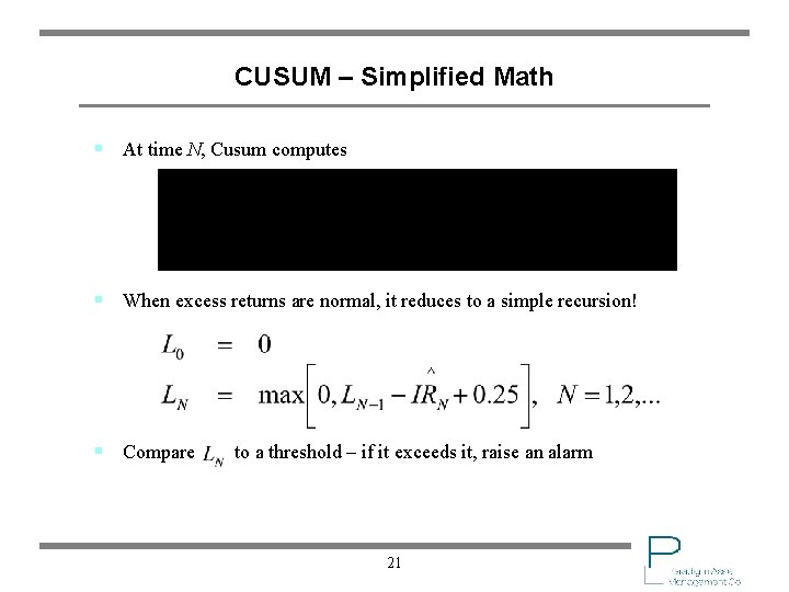
CUSUM – Simplified Math § At time N, Cusum computes § When excess returns are normal, it reduces to a simple recursion! § Compare to a threshold – if it exceeds it, raise an alarm 21

CUSUM: Algorithmic Description § Step 0: Initialize Tracking Error, set likelihood ratio to 0 § Each time a new return is recorded, perform the following 3 steps – Step 1: Compute excess return, tracking error and information ratio – Step 2: Update the likelihood ratio using simple recursion – Step 3: Compare the likelihood ratio to a threshold • If it does not exceed the threshold, do nothing, wait for the next return • If it exceeds the threshold, raise an alarm, launch an investigation § If investigation suggests that this is a false alarm – Reset likelihood ratio to 0, restart CUSUM § If evidence suggests that a problem exists, take corrective action 22

CUSUM: Setting The Threshold For An Alarm § Must make a trade-off between detection speed and rate of false alarms § Our choices: – Average time to detect a bad manager: 41 months (10 x faster than t-test) – Average time between false alarms for a good manager: 84 months 23

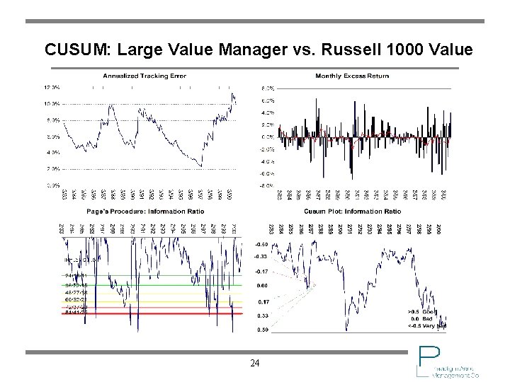
CUSUM: Large Value Manager vs. Russell 1000 Value 24

CUSUM: Large Value Manager vs. Russell 1000 Value 25

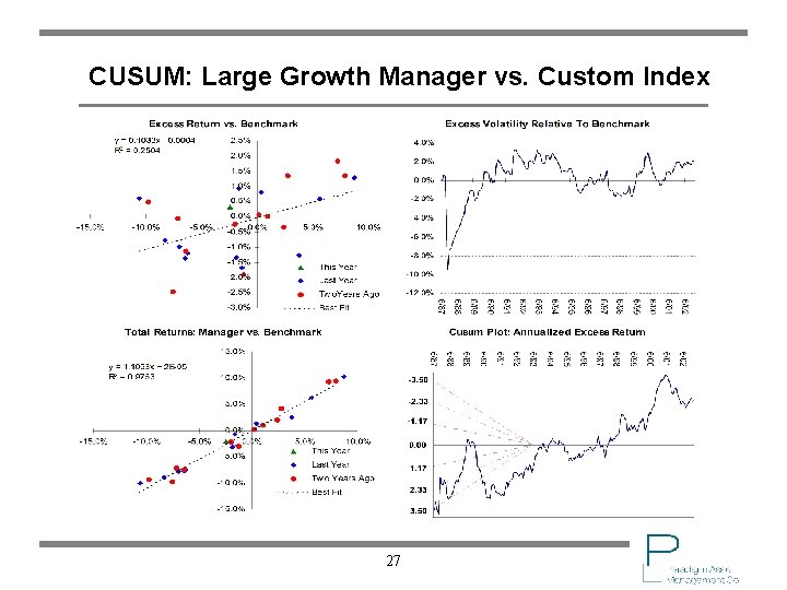
CUSUM: Large Growth Manager vs. Custom Index 26

CUSUM: Large Growth Manager vs. Custom Index 27

CUSUM: Strengths § Detects underperformance exceptionally fast – Provably optimal, though proof is very hard § Robust to distributions of returns – Likelihood ratio is weakly dependent on return distribution § Adapts to changes in tracking error – Can use it in any asset class without modification § Very easy to implement – Can be done in Excel or in specialized SPC packages 28

CUSUM: Limitations § Thoughtless use can lead users astray – Wrong benchmark is the most common error § Does not provide a causal explanation for a change in performance – Use it to launch investigations, not as a hire/fire tool § Somewhat sensitive to correlation – If correlation coefficient < 0. 5, just raise threshold – For higher correlation coefficients, must rework the recursion – Best solution: use the right benchmark 29

CUSUM in Practice § Cusum is extraordinarily powerful, but can be abused – Extreme robustness can lead to abuse § Do not run it on autopilot as a hire / fire tool – It is a monitoring and investigative tool § Run additional tests when an alarm is raised – Determine why the manager underperformed § Ensure that the benchmark is good – Excess returns should be uncorrelated § Thresholds are chosen to work well in practice – Don’t second guess Cusum before an alarm is raised 30

Summary § Cusum detects underperformance rapidly – Over 10 times faster than standard techniques § Very powerful and reliable technique – Extremely robust- works across styles & asset classes – Very few false alarms in practice – Focuses attention on managers who require it § In daily use at a number of large institutions – Plan sponsors, asset managers and consultants – Used to monitor over $500 billion in actively managed assets 31