Money Interest and Income Chapter 11 Introduction Money

Money, Interest, and Income Chapter #11

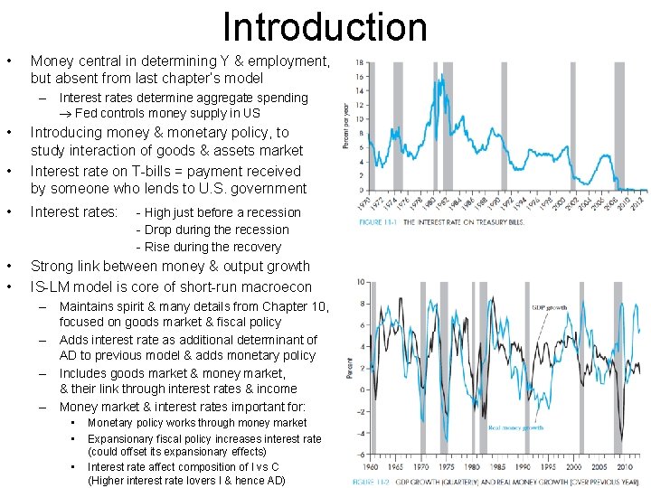
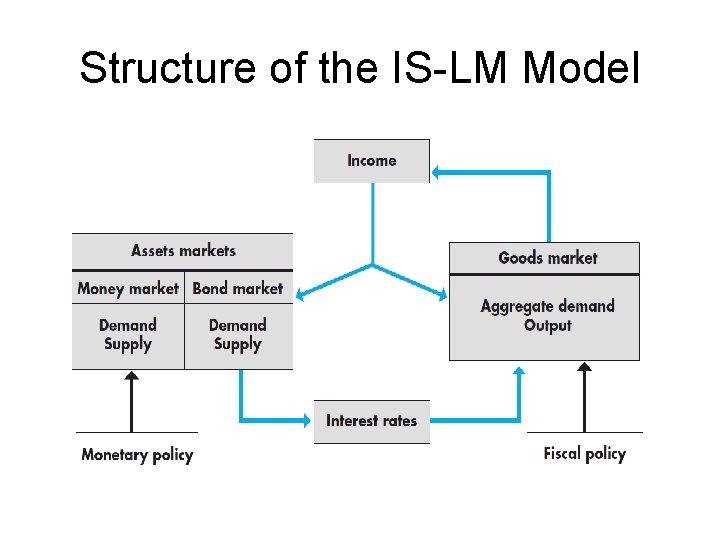
Introduction • Money central in determining Y & employment, but absent from last chapter’s model – Interest rates determine aggregate spending Fed controls money supply in US • • Introducing money & monetary policy, to study interaction of goods & assets market Interest rate on T-bills = payment received by someone who lends to U. S. government • Interest rates: • • Strong link between money & output growth IS-LM model is core of short-run macroecon - High just before a recession - Drop during the recession - Rise during the recovery – Maintains spirit & many details from Chapter 10, focused on goods market & fiscal policy – Adds interest rate as additional determinant of AD to previous model & adds monetary policy – Includes goods market & money market, & their link through interest rates & income – Money market & interest rates important for: • • • Monetary policy works through money market Expansionary fiscal policy increases interest rate (could offset its expansionary effects) Interest rate affect composition of I vs C (Higher interest rate lovers I & hence AD)

Structure of the IS-LM Model

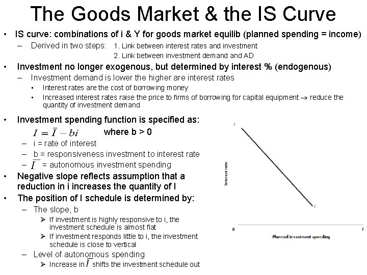
The Goods Market & the IS Curve • IS curve: combinations of i & Y for goods market equilib (planned spending = income) – Derived in two steps: 1. Link between interest rates and investment 2. Link between investment demand AD • Investment no longer exogenous, but determined by interest % (endogenous) – Investment demand is lower the higher are interest rates • • • Interest rates are the cost of borrowing money Increased interest rates raise the price to firms of borrowing for capital equipment reduce the quantity of investment demand Investment spending function is specified as: where b > 0 – i = rate of interest – b = responsiveness investment to interest rate – = autonomous investment spending • • Negative slope reflects assumption that a reduction in i increases the quantity of I The position of I schedule is determined by: – The slope, b Ø If investment is highly responsive to i, the investment schedule is almost flat Ø If investment responds little to i, the investment schedule is close to vertical – Level of autonomous spending Ø Increase in shifts the investment schedule out

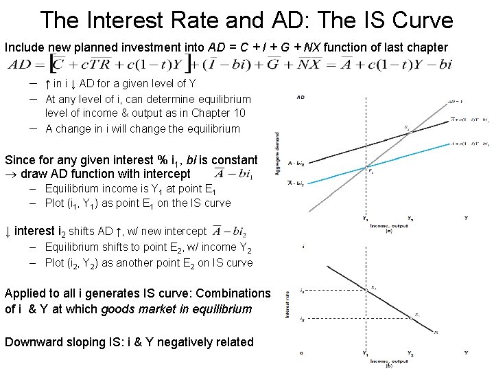
The Interest Rate and AD: The IS Curve Include new planned investment into AD = C + I + G + NX function of last chapter ─ ↑ in i ↓ AD for a given level of Y ─ At any level of i, can determine equilibrium level of income & output as in Chapter 10 ─ A change in i will change the equilibrium Since for any given interest % i 1, bi is constant draw AD function with intercept – Equilibrium income is Y 1 at point E 1 – Plot (i 1, Y 1) as point E 1 on the IS curve ↓ interest i 2 shifts AD ↑, w/ new intercept – Equilibrium shifts to point E 2, w/ income Y 2 – Plot (i 2, Y 2) as another point E 2 on IS curve Applied to all i generates IS curve: Combinations of i & Y at which goods market in equilibrium Downward sloping IS: i & Y negatively related

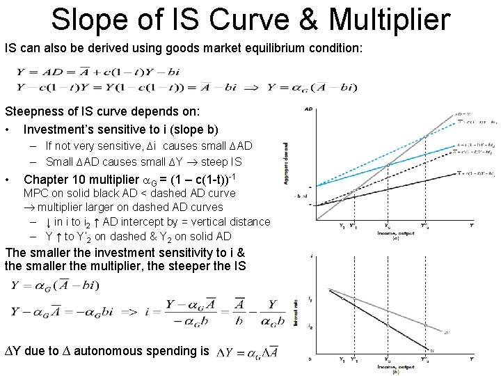
Slope of IS Curve & Multiplier IS can also be derived using goods market equilibrium condition: Steepness of IS curve depends on: • Investment’s sensitive to i (slope b) – If not very sensitive, ∆i causes small ∆AD – Small ∆AD causes small ∆Y steep IS • Chapter 10 multiplier G = (1 – c(1 -t))-1 MPC on solid black AD < dashed AD curve multiplier larger on dashed AD curves – ↓ in i to i 2 ↑ AD intercept by = vertical distance – Y ↑ to Y’ 2 on dashed & Y 2 on solid AD The smaller the investment sensitivity to i & the smaller the multiplier, the steeper the IS ∆Y due to ∆ autonomous spending is

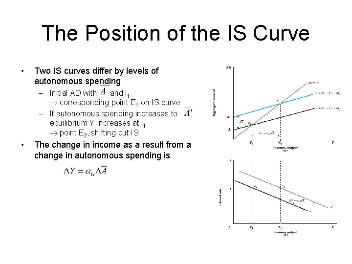
The Position of the IS Curve • Two IS curves differ by levels of autonomous spending – Initial AD with and i 1 corresponding point E 1 on IS curve – If autonomous spending increases to equilibrium Y increases at i 1 point E 2, shifting out IS • , The change in income as a result from a change in autonomous spending is

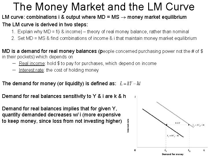
The Money Market and the LM Curve LM curve: combinations i & output where MD = MS money market equilibrium The LM curve is derived in two steps: 1. Explain why MD = f(i & income) – theory of real money balance, rather than nominal 2. Set MD = MS & find combinations of income & i that maintain money market equilibrium MD is a demand for real money balances (people concerned purchasing power not the # of $ in their pockets) which depends on ─ Real income: hold $ to pay for purchases, which depend on income ─ Interest rate: the cost of holding money The demand for money (or liquidity) is defined as: Demand for real balances sensitivity to Y & i are k & h Demand for real balances implies that for given Y, quantity demanded decreases w/ i (more expensive to keep money, since loss from not investing higher)

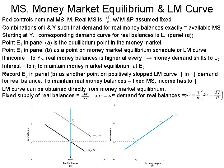
MS, Money Market Equilibrium & LM Curve Fed controls nominal MS, M. Real MS is , w/ M &P assumed fixed Combinations of i & Y such that demand for real money balances exactly = available MS Starting at Y 1, corresponding demand curve for real balances is L 1 (panel (a)) Point E 1 in panel (a) is the equilibrium point in the money market Point E 1 in panel (b) as a point on money market equilibrium schedule or LM curve If income ↑ to Y 2, real money balances is higher at every i money demand shifts to L 2 Interest ↑ to i 2 to maintain money market equilibrium at E 2 Record E 2 in panel (b) as another point on positively slopped LM curve: ↑ in i ↓ demand for real balance. To maintain real money balances = fixed MS, income has to ↑ LM curve can be obtained directly from money market equilibrium: Fixed supply of real balances = = demand for real balances =>

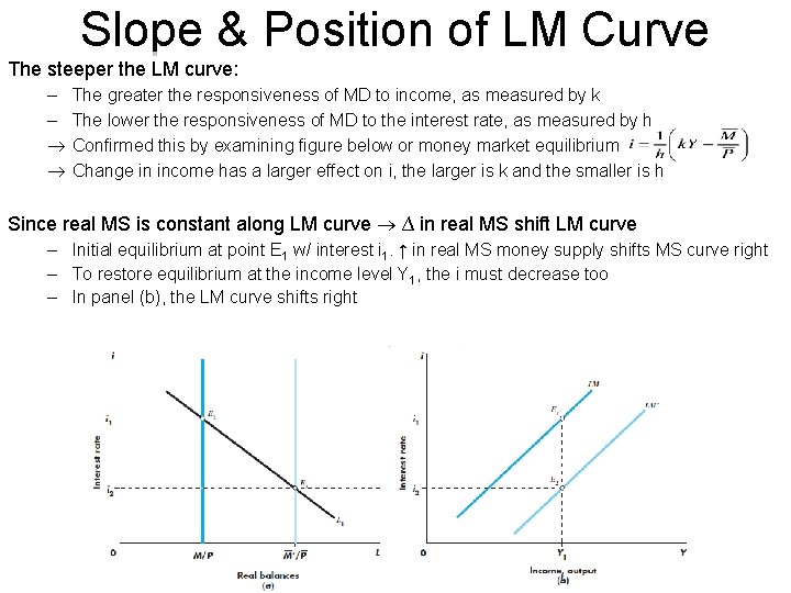
Slope & Position of LM Curve The steeper the LM curve: – – The greater the responsiveness of MD to income, as measured by k The lower the responsiveness of MD to the interest rate, as measured by h Confirmed this by examining figure below or money market equilibrium Change in income has a larger effect on i, the larger is k and the smaller is h Since real MS is constant along LM curve ∆ in real MS shift LM curve – Initial equilibrium at point E 1 w/ interest i 1. ↑ in real MS money supply shifts MS curve right – To restore equilibrium at the income level Y 1, the i must decrease too – In panel (b), the LM curve shifts right

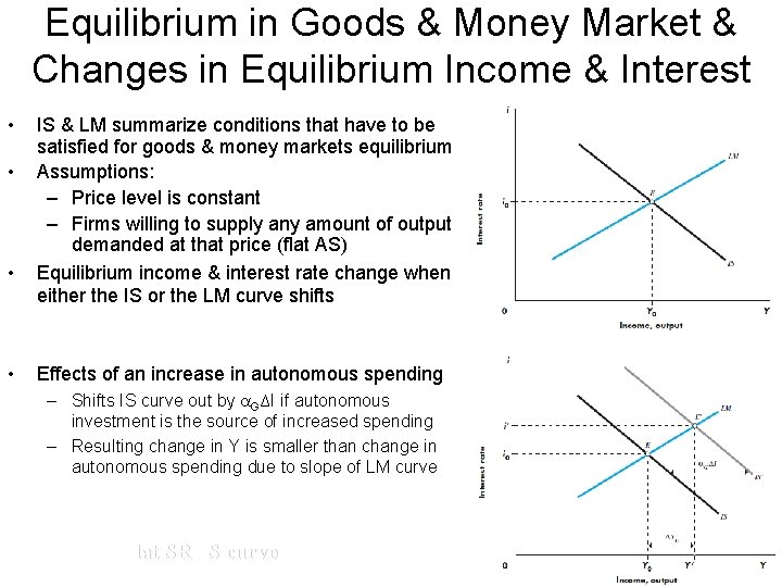
Equilibrium in Goods & Money Market & Changes in Equilibrium Income & Interest • • IS & LM summarize conditions that have to be satisfied for goods & money markets equilibrium Assumptions: – Price level is constant – Firms willing to supply any amount of output demanded at that price (flat AS) Equilibrium income & interest rate change when either the IS or the LM curve shifts Effects of an increase in autonomous spending – Shifts IS curve out by G∆I if autonomous investment is the source of increased spending – Resulting change in Y is smaller than change in autonomous spending due to slope of LM curve Flat SRAS curve

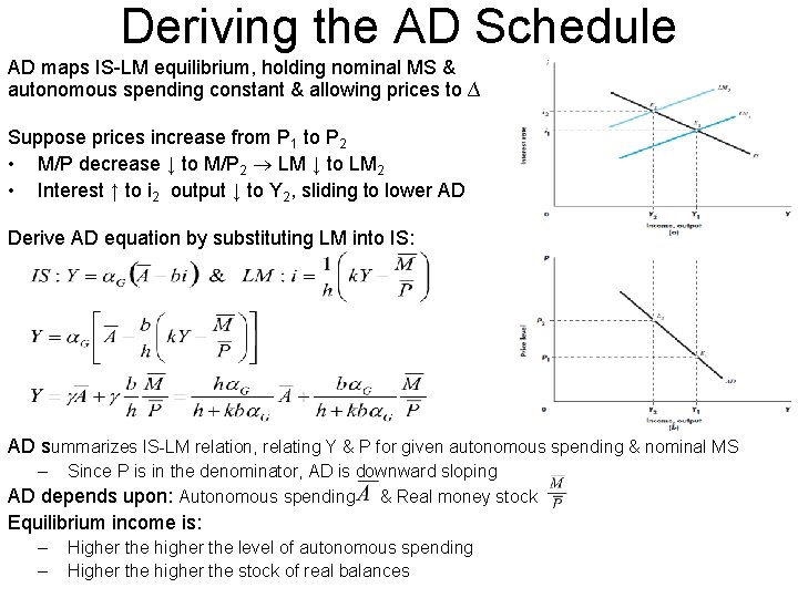
Deriving the AD Schedule AD maps IS-LM equilibrium, holding nominal MS & autonomous spending constant & allowing prices to ∆ Suppose prices increase from P 1 to P 2 • M/P decrease ↓ to M/P 2 LM ↓ to LM 2 • Interest ↑ to i 2 output ↓ to Y 2, sliding to lower AD Derive AD equation by substituting LM into IS: AD summarizes IS-LM relation, relating Y & P for given autonomous spending & nominal MS – Since P is in the denominator, AD is downward sloping AD depends upon: Autonomous spending & Real money stock Equilibrium income is: – – Higher the higher the level of autonomous spending Higher the higher the stock of real balances