Monetary and Fiscal Policy Chapter 12 Copyright 2014

Monetary and Fiscal Policy Chapter #12 Copyright © 2014 Mc. Graw-Hill Education. All rights reserved. No reproduction or distribution without the prior written consent of Mc. Graw-Hill Education.

Introduction • In this chapter we use the IS-LM model developed in Chapter 11 to show monetary and fiscal policy work – Fiscal policy has its initial impact in the goods market – Monetary policy has its initial impact mainly in the assets markets Because the goods and assets markets are interconnected, both fiscal and monetary policies have effects on both the level of output and interest rates Expansionary/contractionary monetary policy moves the LM curve to the right/left Expansionary/contractionary fiscal policy moves the IS curve to the right/left 12 -2

Monetary Policy • • The Federal Reserve is responsible for monetary policy in the U. S. conducted mainly through open market operations Open market operations: buying and selling of government bonds ─ Fed buys bonds in exchange for money increases the stock of money (Fig. 12 -3) ─ Fed sells bonds in exchange for money paid by purchasers of the bonds reducing the money stock 12 -3

Monetary Policy • Adjustment to the monetary expansion: – Increase in money supply creates excess supply of money – Public buys other assets – Asset prices increase, yields decrease move to point E 1 – Decline in interest rate results in excess demand for goods – Output expands and move up LM’ schedule 12 -4

Figure shows graphically how an open market purchase works. The initial equilibrium at point E is on the initial LM schedule that corresponds to a real money supply M/P. Now consider an open market purchase by the Fed. This increases the nominal quantity of money and, given the price level, the real quantity of money. As a consequence, the LM schedule will shift to LM’. The new equilibrium will be at point with a lower interest rate and a higher level of income. The equilibrium level of income rises because the open market purchase reduces the interest rate and thereby increases investment spending.

Consider next the process of adjustment to the monetary expansion. At the initial equilibrium point, E, the increase in the money supply creates an excess supply of money to which the public adjusts by trying to buy other assets. In the process, asset prices increase and yields decline. Because money and asset markets adjust rapidly, we move immediately to point E 1, where the money market clears and where the public is willing to hold the larger real quantity of money because the interest rate has declined sufficiently. At point E 1, however, there is an excess demand for goods. The decline in the interest rate, given the initial income level has raised aggregate demand is causing inventories to run down. In response, output expands and we start moving up the schedule.

Why does the interest rate rise during the adjustment process? Because the increase in output raises the demand for money, and the greater demand for money has to be checked by higher interest rates. Thus, the increase in the money stock first causes interest rates to fall as the public adjusts its portfolio and then—as a result of the decline in interest rates—increases aggregate demand.

Adjustment to the monetary expansion At E ESM (L< M/P) → Pbond ↑ → i↓ → I ↑ → Y ↑ → L↑→ i↑ Reach to E’ At E 1 EDG → Y ↑

Transmission Mechanism • Two steps in the transmission mechanism (the process by which changes in monetary policy affect AD): 1. An increase in real balances generates a portfolio disequilibrium – At the prevailing interest rate and level of income, people are holding more money than they want – Portfolio holders attempt to reduce their money holdings by buying other assets changes asset prices and yields – The change in money supply changes interest rates 2. A change in interest rates affects AD 12 -9

The Liquidity Trap • Two extreme cases arise when discussing the effects of monetary policy on the economy first is the liquidity trap – Liquidity trap = a situation in which the public is prepared, at a given interest rate, to hold whatever amount of money is supplied – Implies the LM curve is horizontal changes in the quantity of money do not shift it • Monetary policy has no impact on either the interest rate or the level of income monetary policy is powerless • Possibility of a liquidity trap at low interest rates is a notion that grew out of theories of English economist John Maynard Keynes 12 -10

LM curve is horizontal. h = ∞ ( Para talebi faize tam duyarlı)

The Classical Case • The opposite of the horizontal LM curve (implies that monetary policy cannot affect the level of income) is the vertical LM curve – Demand for money is entirely unresponsive to the interest rate – Recall, the equation for the LM curve is (1) • If h is zero, then there is a unique level of income corresponding to a given real money supply VERTICAL LM CURVE • The vertical LM curve is called the classical case – Rewrite equation (1), with h = 0: (2) • Implies that NGDP depends only on the quantity of money quantity theory of money 12 -12

If h is zero, then corresponding to a given real money supply M/P, there is a unique level of income, which implies that the LM curve is vertical at that level of income. The vertical LM curve is called the classical case. M = k( P x Y) M and P constant. We see that the classical case implies that nominal GDP, P x Y, depends only on the quantity of money. This is the classical quantity theory of money, which argues that the level of nominal income is determined solely by the quantity of money.

The Classical Case • When the LM curve is vertical 1. A given change in the quantity of money has a maximal effect on the level of income 2. Shifts in the IS curve do not affect the level of income • Vertical LM curve implies the comparative effectiveness of monetary policy over fiscal policy – “Only money matters” for the determination of output – Requires that the demand for money be irresponsive to i important issue in determining the effectiveness of alternative policies 12 -14

Fiscal Policy and Crowding Out • The equation for the IS curve is: (3) – The fiscal policy variables, G and t, are within this definition • G is a part of A • t is a part of the multiplier Fiscal policy actions, changes in G and t, affect the IS curve • Suppose G increases – At unchanged interest rates, AD increases – To meet increased demand, output must increase – At each level of the interest rate, equilibrium income must rise by 12 -15

Fiscal Policy and Crowding Out • • If government expenditures increase, equilibrium moves to from E to E” The goods market is in equilibrium at E”, but the money market is not: – Because Y has increased, the demand for money also increases interest rate increases – Firms’ planned investment spending declines and AD falls move up the LM curve to E’ 12 -16

Fiscal Policy and Crowding Out • • Comparing E to E’: increased government spending increases income and the interest rate Comparing E’ to E”: adjustment of interest rates and their impact on AD dampen expansionary effect of increased G – Income increases to Y’ 0 instead of Y” 12 -17

The reason that income rises only to Yo’ rather than to Y’’ is that the rise in the interest rate from io to i’ reduces the level of investment spending. We say that the increase in government spending crowds out investment spending. Crowding out occurs when expansionary fiscal policy causes interest rates to rise, thereby reducing private spending, particularly investment.

THE LIQUIDITY TRAP If the economy is in the liquidity trap, and thus the LM curve is horizontal, an increase in government spending has its full multiplier effect on the equilibrium level of income. There is no change in the interest rate associated with the change in government spending, and thus no investment spending is cut off. There is therefore no dampening of the effects of increased government spending on income. If the LM curve is horizontal, monetary policy has no impact on the equilibrium of the economy and fiscal policy has a maximal effect. Less dramatically, if the demand for money is very sensitive to the interest rate, and thus the LM curve is almost horizontal, fiscal policy changes have a relatively large effect on output and monetary policy changes have little effect on the equilibrium level of output.

THE CLASSICAL CASE AND CROWDING OUT If the LM curve is vertical, an increase in government spending has no effect on the equilibrium level of income and increases only the interest rate. Thus, with a vertical LM curve, an increase in government spending cannot change the equilibrium level of income and raises only the equilibrium interest rate. But if government spending is higher and output is unchanged, there must be an offsetting reduction in private spending. In this case, the increase in interest rates crowds out an amount of private (particularly investment) spending equal to the increase in government spending. Thus, there is full crowding out if the LM curve is vertical.

Full Crowding Out

MONETARY ACCOMMODATION OF FISCAL EXPANSION Monetary policy is accommodating when, in the course of a fiscal expansion, the money supply is increased in order to prevent interest rates from increasing. Monetary accommodation is also referred to as monetizing budget deficits, meaning that the Federal Reserve prints money to buy the bonds with which the government pays for its deficit. When the Fed accommodates a fiscal expansion, both the IS and the LM schedules shift to the right. Output will clearly increase, but interest rates need not rise. Accordingly, there need not be any adverse effects on investment.

MONETARY ACCOMMODATION OF FISCAL EXPANSION

The Composition of Output and the Policy Mix • • • Table 12 -2 summarizes effects of expansionary monetary and fiscal policy on output and the interest rate Monetary policy operates by stimulating interest-responsive components of AD Fiscal policy operates through G and t impact depends upon what goods the government buys and what taxes and transfers it changes 12 -24

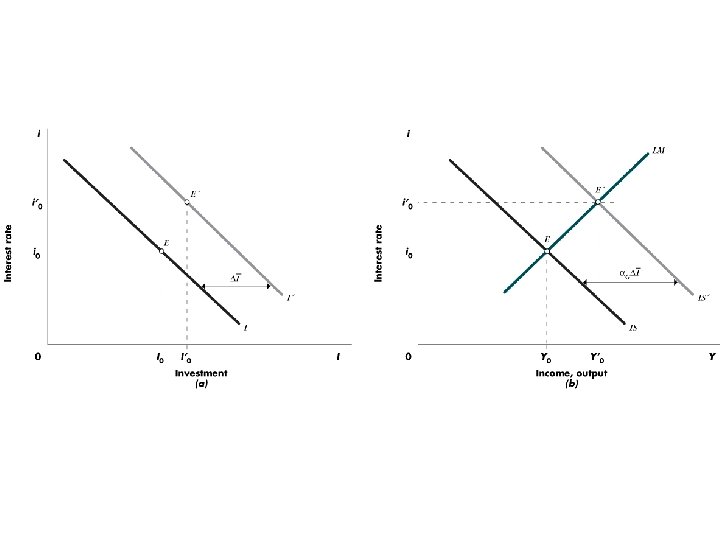
AN INVESTMENT SUBSIDY Both an income tax cut and an increase in government spending raise the interest rate and reduce investment spending. However, it is possible for the government to raise investment spending through an investment subsidy. When the government subsidizes investment, it essentially pays part of the cost of each firm’s investment. An investment subsidy shifts the investment schedule to the right. At each interest rate, firms now plan to invest more. With investment spending higher, aggregate demand increases.

In panel (b), the IS schedule shifts by the amount of the multiplier times the increase in autonomous investment brought about by the subsidy. The new equilibrium is at point E’, where goods and money markets are again in balance. But note now that although interest rates have risen, we see, in panel (a), that investment is higher. Investment is at the level up I 0’ from I 0. The interest rate increase dampens but does not reverse the impact of the investment subsidy. This is an example in which both consumption, induced by higher income, and investment rise as a consequence of expansionary fiscal policy.

Alternative Fiscal Policies Interest Rate Consumption Investment GDP Income Tax Cut + + - + Government Spending + + - + Investment Subsidy + +

The Composition of Output and the Policy Mix Policy problem of reaching full employment output, Y*, for an economy that is initially at point E, with unemployment Choices: • 1. Fiscal policy expansion, moving to point E 1, with higher income and higher interest rates 2. Monetary policy expansion, resulting in full employment with lower interest rates at point E 2 3. A mix of fiscal expansion and accommodating monetary policy resulting in an intermediate position 12 -29

The Composition of Output and the Policy Mix • • Policies all increase output, but significantly different impact on sectors of the economy problem of political economy Who should be the primary beneficiary of expansion? – An expansion through a decline in interest rates and increased investment spending? – An expansion through a tax cut and increased personal consumption? – An expansion in the form of an increase in the size of the government? 12 -30