MondayTuesday Solutions Thermodynamics of aqueous solutions Saturation indices

Monday-Tuesday • Solutions – Thermodynamics of aqueous solutions – Saturation indices • • • Mineral equilibria Cation exchange Surface complexation Advective transport Diffusive transport Acid mine drainage 1

Processes that Control Major Element Chemistry 1. Carbonate reactions 2. Ion exchange 3. Organic carbon oxidation O 2/Nitrate reduction Iron oxyhydroxide reduction Sulfate reduction Methanogenesis 4. Gypsum dissolution 5. Pyrite oxidation 6. Seawater evaporation 7. Silicate weathering

Processes that Control Minor Element Chemistry 1. Redox Oxyanions Trace metals Nitrate 2. Surface complexation Phosphate Oxyanions Trace metals 3. Cation exchange 4. Solid solutions 5. Minerals

PHREEQC Programs • PHREEQC Version 3 – PHREEQC: Batch with Charting – Phreeqc. I: GUI with Charting – IPhreeqc: Module for programming and scripting • PHAST – – Serial—soon to be Multithreaded Parallel—MPI for transport and chemistry TVD (not done) 4 Windows—GUI just accepted • WEBMOD-Watershed reactive transport 4

Solution Definition and Speciation Calculations SO 4 Ca Na Mg Cl Fe HCO 3 Inverse Modeling Saturation Indices Speciation calculation Reactions Transport 5

SOLUTION: Seawater, ppm Constituent p. H pe Temperature Ca Mg Na K Fe Alkalinity as HCO 3 Cl SO 4 Value 8. 22 8. 45 10 412. 3 1291. 8 10768 399. 1. 002 141. 682 19353 2712 6

Periodic_table. bmp 7

Initial Solution 1. Questions 1. What is the approximate molality of Ca? 2. What is the approximate alkalinity in meq/kgw? 3. What is the alkalinity concentration in mg/kgs as Ca. CO 3? 4. What effect does density have on the calculated molality? PHREEQC results are always moles or molality 8

Initial Solution 1. For most waters, we can assume most of the mass in solution is water. Mass of water in 1 kg seawater ~ 1 kg. 1. 412/40 ~ 10 mmol/kgw ~ 0. 01 molal 2. 142/61 ~ 2. 3 meq/kgw ~ 0. 0023 molal 3. 2. 3*50 ~ 116 mg/kgw as Ca. CO 3 4. None, density will only be used when concentration is specified as per liter. 9

Default Gram Formula Mass Element/Redox State Default “as” phreeqc. dat/wateq 4 f. dat Alkalinity Ca. CO 3 C, C(4) HCO 3 CH 4 NO 3 - N NH 4+ N PO 4 P Si Si. O 2 SO 4 Default GFW is defined in 4 th field of SOLUTION_MASTER_SPECIES in database file. 10

Databases • Ion association approach – – – – Phreeqc. dat—simplest (subset of Wateq 4 f. dat) Amm. dat—same as phreeqc. dat, NH 3 is separated from N Wateq 4 f. dat—more trace elements Minteq. dat—translated from minteq v 2 Minteq. v 4. dat—translated from minteq v 4 Llnl. dat—most complete set of elements, temperature dependence Iso. dat—(in development) thermodynamics of isotopes • Pitzer specific interaction approach – Pitzer. dat—Specific interaction model (many parameters) • SIT specific interaction theory – Sit. dat—Simplified specific interaction model (1 parameter) 11

PHREEQC Databases Other data blocks related to speciation SOLUTION_MASTER_SPECIES—Redox states and gram formula mass SOLUTION_SPECIES—Reaction and log K PHASES—Reaction and log K 12

Solutions • Required for all PHREEQC calculations • SOLUTION and SOLUTION _SPREAD – – – Units p. H pe Charge balance Phase boundaries • Saturation indices – Useful minerals – Identify potential reactants 13

What is a speciation calculation? • Input: – p. H – pe – Concentrations • Equations: – Mass-balance—sum of the calcium species = total calcium – Mass-action—activities of products divided by reactants = constant – Activity coefficients—function of ionic strength • Output – Molalities, activities – Saturation indices 14

Mass-Balance Equations Analyzed concentration of sulfate = (SO 4 -2) + (Mg. SO 40) + (Na. SO 4 -) + (Ca. SO 40) + (KSO 4 -) + (HSO 4 -) + (Ca. HSO 4+) + (Fe(SO 4)2 -) + (Fe. HSO 4+2) () indicates molality 15

Mass-Action Equations Ca+2 + SO 4 -2 = Ca. SO 40 [] indicates activity 16

Activity WATEQ activity coefficient Davies activity coefficient 17

Uncharged Species bi, called the Setschenow coefficient Value of 0. 1 used in phreeqc. dat, wateq 4 f. dat. 18

Pitzer Activity Coefficients ma concentration of anion mc concentration of cation Ion specific parameters F function of ionic strength, molalities of cations and anions 19

SIT Activity Coefficients mk concentrations of ion Interaction parameter A = 0. 51, B = 1. 5 at 25 C 20

Aqueous Models Ion association – Pros • Data for most elements (Al, Si) • Redox – Cons • • Ionic strength < 1 Best only in Na, Cl medium Inconsistent thermodynamic data Temperature dependence 21

Aqueous Models • Pitzer specific interaction – Pros • High ionic strength • Thermodynamic consistency for mixtures of electrolytes – Cons • • Limited elements Little if any redox Difficult to add elements Temperature dependence 22

Aqueous Models • SIT – Pros • Possibly better for higher ionic strength than ion association • Many fewer parameters • Redox • Actinides – Cons • Poor results for gypsum/Na. Cl in my limited testing • Temperature dependence • Consistency? 23

Phreeqc. I: SOLUTION Data Block 24

Number, p. H, pe, Temperature 25

Solution Composition Set units! Default is mmol/kgw Select elements Set concentrations “As”, special units Click when done 26

Run Speciation Calculation Run Select files 27

Seawater Exercise A. Use phreeqc. dat to run a speciation calculation for file seawater. pqi B. Use file seawaterpitzer. pqi or copy input to a new buffer • • Ctrl-a (select all) Ctrl-c (copy) File->new or ctrl-n (new input file) Ctrl-v (paste) Units are ppm Constituent p. H p. E Temperature Ca Mg Na K Fe Alkalinity as HCO 3 Cl SO 4 Value 8. 22 8. 45 10 412. 3 1291. 8 10768 399. 1. 002 141. 682 19353 2712 28

Ion Association Model Results 29

Results of 2 Speciation Calculations Tile Ion Association Pitzer 30

Questions 1. Write the mass-balance equation for calcium in seawater for each database. 2. What fraction of the total is Ca+2 ion for each database? 3. What fraction of the total is Fe+3 ion for each database? 4. What are the log activity and log activity coefficient of CO 3 -2 for each database? 5. What is the saturation index of calcite for each database? 31

Initial Solution 2. Answers () indicates molality 1 a. Ca(total)= 1. 066 e-2 = (Ca+2) + (Ca. SO 4) + (Ca. HCO 3+) + (Ca. CO 3) + (Ca. OH+) + (Ca. HSO 4+) 1 b. Ca(total) = 1. 066 e-2 = (Ca+2) + (Ca. CO 3) 2 a. 9. 5/10. 7 ~ 0. 95 2 b. 1. 063/1. 066 ~ 1. 0 3 a. 3. 509 e-019 / 3. 711 e-008 ~ 1 e-11 3 b. No Fe+3 ion. 4 a. log activity CO 3 -2 = -5. 099; log gamma CO 3 -2 = -0. 68 4 b. log activity CO 3 -2 = -5. 091; log gamma CO 3 -2 = -1. 09 5 a. SI(calcite) = 0. 76 5 b. SI(calcite) = 0. 70 32

SATURATION INDEX The thermodynamic state of a mineral relative to a solution IAP is ion activity product K is equilibrium constant 33

SATURATION INDEX SI < 0, Mineral should dissolve SI > 0, Mineral should precipitate SI ~ 0, Mineral reacts fast enough to maintain equilibrium Maybe – Kinetics – Uncertainties 34

Rules for Saturation Indices • Mineral cannot dissolve if it is not present • If SI < 0 and mineral is present—the mineral could dissolve, but not precipitate • If SI > 0—the mineral could precipitate, but not dissolve • If SI ~ 0—the mineral could dissolve or precipitate to maintain equilibrium 35

Saturation Indices • SI(Calcite) • SI(CO 2(g)) = log(PCO 2) 36

Useful Mineral List Minerals that may react to equilibrium relatively quickly 37

• Files (double click to edit) Data Tree – Simulation (END) • Keywords (double click to edit) – Data 38

Edit Screen • Text editor 39

Tree Selection • • • Input Output Database Errors Pf. W 40

Keyword Data Blocks Also right click in data tree—Insert keyword 41

Pf. W Style 42

Total Inorganic Carbon • Number of moles of carbon of valence 4 Alkalinity • Approximately HCO 3 - + 2 x. CO 3 -2 + OH- - H+ • Alkalinity is independent of PCO 2 43

SOLUTION_SPREAD 44

Carbon and Alkalinity solution_spread. pqi SOLUTION_SPREAD SELECTED_OUTPUT USER_GRAPH 45

Carbon Speciation and Alkalinity 46

p. H and pe Keywords SOLUTION—Solution composition END—End of a simulation USE—Reactant to add to beaker REACTION—Specified moles of a reaction USER_GRAPH—Charting 47

SOLUTION, mmol/kgw Constituent p. H pe Temperature Alkalinity Na Value 7 4 25 1 1 charge END 48

USE Solution 1 REACTION CO 2 1. 0 1, 100, 1000 mmol USER_GRAPH -axis_titles "CO 2 Added, mmol" "p. H" "Alkalinity" -axis_scale x_axis auto log -axis_scale sy_axis 0 0. 002 -start 10 GRAPH_X rxn 20 GRAPH_Y -LA("H+") 30 GRAPH_SY ALK -end 49

Input file p. H. pqi SOLUTION 1 temp 25 p. H 7 pe 4 redox pe units mmol/kgw density 1 Alkalinity 1 Na 1 charge -water 1 # kg END USE solution 1 REACTION 1 CO 2 1 1 10 1000 millimoles USER_GRAPH 1 -axis_titles "CO 2 Added, mmol" "p. H" "Alkalinity" -axis_scale x_axis auto log -axis_scale sy_axis 0 0. 002 -start 10 GRAPH_X rxn 20 GRAPH_Y -LA("H+") 30 GRAPH_SY ALK -end END 50

p. H is the ratio of HCO 3 - to CO 2(aq) Alkalinity is independent of PCO 2 51

What is p. H? p. H = 6. 3 + log[(HCO 3 -)/(CO 2)] p. H = 10. 3 + log[(CO 3 -2)/(HCO 3 -)] p. H = log. K + log[(PO 4 -3)/(HPO 4 -2)] Questions 1. How does the p. H change when CO 2 degasses during an alkalinity titration? 2. How does p. H change when plankton respire CO 2? 3. How does p. H change when calcite dissolves? 52

SOLUTION, mmol/kgw Constituent p. H pe Temperature Fe(3) Cl Value 2 4 25 1 1 charge END 53

USE Solution 1 REACTION Fe. Cl 2 1. 0 1, 100, 1000 mmol USER_GRAPH -axis_titles "Fe. Cl 2 Added, mmol" "pe" "" -axis_scale x_axis auto log -start 10 GRAPH_X rxn 20 GRAPH_Y -LA("e-") -end 54

Input file SOLUTION 1 temp 25 p. H 3 pe 4 redox pe units mmol/kgw density 1 Cl 1 charge Fe(3) 1 -water 1 # kg END USE solution 1 REACTION 1 Fe. Cl 2 1 1 10 1000 millimoles USER_GRAPH 1 -axis_titles "Fe. Cl 2 Added, mmol" "pe" "" -axis_scale x_axis auto log -start 10 GRAPH_X rxn 20 GRAPH_Y -LA("e-") -end END 55

pe 56

What is pe? Fe+2 = Fe+3 + epe = log( [Fe+3]/[Fe+2] ) + 13 HS- + 4 H 2 O = SO 4 -2 + 9 H+ + 8 epe = log( [SO 4 -2]/[HS-] ) – 9/8 p. H + 4. 21 N 2 + 6 H 2 O = 2 NO 3 - + 12 H+ + 10 epe = 0. 1 log( [NO 3 -]2/[N 2] ) – 1. 2 p. H + 20. 7 pe = 16. 9 Eh, Eh in volts (platinum electrode measurement) 57

Redox and pe in SOLUTION Data Blocks • When do you need pe for SOLUTION? – To distribute total concentration of a redox element among redox states [e. g. Fe to Fe(2) and Fe(3)] – A few saturation indices with e- in dissociation reactions • Pyrite • Native sulfur • Manganese oxides • Can use a redox couple Fe(2)/Fe(3) in place of pe • Rarely, pe = 16. 9 Eh. (25 C and Eh in Volts). • pe options can only be applied to speciation calculations; thermodynamic pe is used for all other calculations 58

Iron Speciation with Phree. Plot 59

Redox Elements Element Redox state Species Carbon C(4) CO 2 Iron Fe(3) Fe+3 C(-4) CH 4 Fe(2) Fe+2 S(6) SO 4 -2 Manganese Mn(2) Mn+2 S(-2) HS- Arsenic As(5) As. O 4 -3 N(5) NO 3 - As(3) As. O 3 -3 N(3) NO 2 - U(6) UO 2+2 N(0) N 2 U(4) U+4 N(-3) NH 4+ Cr(6) Cr. O 4 -2 O(0) O 2 Cr(3) Cr+3 O(-2) H 2 O Se(6) Se. O 4 -2 H 2 O Se(4) Se. O 3 -2 H 2 Se(-2) HSe- Sulfur Nitrogen Oxygen Hydrogen H(1) H(0) Uranium Chromium Selenium 60

Seawater Initial Solution Fe total was entered. How were Fe(3) and Fe(2) concentrations calculated? For initial solutions For “reactions” 61

Final thoughts on pe • pe sets ratio of redox states • Some redox states are measured directly: – – NO 3 -, NO 2 -, NH 3, N 2(aq) SO 4 -2, HSO 2(aq) Sometimes Fe, As • Others can be assumed: – – – Fe, always Fe(2) except at low p. H Mn, always Mn(2) As, consider other redox elements Se, consider other redox elements U, probably U(6) V, probably V(5) 62

Berner’s Redox Environments • • Oxic Suboxic Sulfidic Methanic Thorstenson (1984) 63

64

Parkhurst and others (1996) 65

Summary SOLUTION and SOLUTION _SPREAD – – – Units p. H—ratio of HCO 3/CO 2 pe—ratio of oxidized/reduced valence states Charge balance Phase boundaries • Saturation indices – Uncertainties – Useful minerals • Identify potential reactants 66

Summary Aqueous speciation model – Mole-balance equations—Sum of species containing Ca equals total analyzed Ca – Aqueous mass-action equations—Activity of products over reactants equal a constant Activity coefficient model – • • – Ion association with individual activity coefficients Pitzer specific interaction approach SI=log(IAP/K) 67

PHREEQC: Reactions in a Beaker SOLUTION MIX + REACTION_TEMPERATURE SOLUTION EXCHANGE SURFACE REACTION BEAKER EQUILIBRIUM_ PHASES EQUILIBRIUM _PHASES EXCHANGE SURFACE KINETICS GAS_PHASE REACTION_PRESSURE GAS_PHASE 68

Reaction Simulations • SOLUTION, SOLUTION_SPREAD, MIX, USE solution, or USE mix Equilibrium EQUILIBRIUM_PHASES EXCHANGE SURFACE SOLID_SOLUTION GAS_PHASE REACTION_TEMPERATURE REACTION_PRESSURE Nonequilibrium • END KINETICS REACTION 69

Calculate the SI of Calcite in Seawater at Pressures from 100 to 1000 atm 70

Keywords SOLUTION 1 END USE solution 1 REACTION_PRESSURE USER_GRAPH END 71

USE—Item on shelf Item number on shelf To the beaker 72

USE All of these Reactants are Numbered • • SOLUTION • REACTION EQUILIBRIUM_PHASES • REACTION_PRESSURE EXCHANGE • REACTION_TEMPERATURE GAS_PHASE KINETICS SOLID_SOLUTIONS SURFACE 73

REACTION_PRESSURE • List of pressures 100 200 300 400 500 600 700 800 900 1000 Or • Range of pressure divided equally 1000 in 10 steps 74

USER_GRAPH 10 GRAPH_X PRESSURE 20 GRAPH_Y SI(“Calcite”) 30 GRAPH_SY expr • Expressions are defined with Basic functions • Basic—+-*/, SIN, COS, EXP, … • PHREEQC—PRESSURE, SI(“Calcite”), MOL(“Cl-”), TOT(“Cl-”), -LA(“H+”), … 75

Plot the SI of Calcite with Temperature Seawater-p. pqi 76

SI Calcite for Seawater with P 77

Arsenic in the Central Oklahoma Aquifer • Arsenic mostly in confined part of aquifer • Arsenic associated with high p. H • Flow: – Unconfined – Confined – Unconfined 78

Geochemical Reactions • Brine initially fills the aquifer • Calcite and dolomite equilibrium • Cation exchange – 2 Na. X + Ca+2 = Ca. X 2 + 2 Na+ – 2 Na. X + Mg+2 = Mg. X 2 + 2 Na+ • Surface complexation Hfo-HAs. O 4 - + OH- = Hfo. OH + HAs. O 4 -2 79

More Reactions and Keywords EQUILIBRIUM_PHASES SAVE EXCHANGE SURFACE 80

EQUILIBRIUM_PHASES Minerals and gases that react to equilibrium Calcite reaction Ca. CO 3 = Ca+2 + CO 3 -2 Equilibrium K = [Ca+2][CO 3 -2]

EQUILIBRIUM_PHASES Data Block • Mineral or gas • Saturation state • Amount Example EQUILIBRIUM_PHASES 5: CO 2 Calcite Dolomite Fe(OH)3 Log PCO 2 = -2, equilibrium 10 moles 1 moles 0 moles

Let’s Make a Carbonate Groundwater • SOLUTION—Pure water or rain • EQUILIBRIUM_PHASES – CO 2(g), SI -1. 5, moles 10 – Calcite, SI 0, moles 0. 1 – Dolomite, SI 0, moles 1. 6 • SAVE solution 0 83

Oklahoma Rainwater x 20 Ignoring NO 3 - and NH 4+ SOLUTION 0 20 x precipitation p. H 4. 6 pe 4. 0 O 2(g) -0. 7 temp 25. units mmol/kgw Ca 0. 191625 Mg 0. 035797 Na 0. 122668 Cl 0. 133704 C 0. 01096 S 0. 235153 charge 84

Limestone Groundwater 85

Brine • Oil field brine 86

SOLUTION Data Block • SOLUTION 1: Oklahoma Brine units mol/kgw p. H 5. 713 temp 25. Ca 0. 4655 Mg 0. 1609 Na 5. 402 Cl 6. 642 C 0. 00396 S 0. 004725 As 0. 03 (ug/kgw)

Ion Exchange Calculations (#1) • Layers of clays have a net negative charge • Exchanger has a fixed CEC, cation exchange capacity, based on charge deficit • Small cations (Ca+2, Na+, NH 4+, Sr+2, Al+3) fit in the interlayers • PHREEQC “speciates” the “exchanged species” on the exchange sites either: – Initial Exchange Calculation: adjusting sorbed concentrations in response to a fixed aqueous composition – Reaction Calculation: adjusting both sorbed and aqueous compositions.

Ion Exchange (#2) • PHREEQC uses 3 keywords to define exchange processes – EXCHANGE_MASTER_SPECIES (component data) – EXCHANGE_SPECIES (species thermo. data) – EXCHANGE • First 2 are found in phreeqc. dat and wateq 4 f. dat (for component X- and exchange species from Appelo) but can be modified in user-created input files. • Last is user-specified to define amount and composition of an “exchanger” phase.

Ion Exchange (#3) • “SAVE” and “USE” keywords can be applied to “EXCHANGE” phase compositions. • Amount of exchanger (eg. moles of X-) can be calculated from CEC (cation exchange capacity, usually expressed in meq/100 g of soil) where: where sw is the specific dry weight of soil (kg/L of soil), q is the porosity and r. B is the bulk density of the soil in kg/L. (If sw = 2. 65 & q = 0. 3, then X- = CEC/16. 2) • CEC estimation technique (Breeuwsma, 1986): CEC (meq/100 g) = 0. 7 (%clay) + 3. 5 (%organic carbon) (cf. Glynn & Brown, 1996; Appelo & Postma, 2005, p. 247)

EXCHANGE Cation exchange composition Reaction: Ca+2 + 2 Na. X = Ca. X 2 + 2 Na+ Equilibrium:

EXCHANGE Data Block • Exchanger name • Number of exchange sites • Chemical composition of exchanger Example EXCHANGE 15: Ca. X 2 Na. X Often X 0. 05 moles (X is defined in databases) 0. 05 moles 0. 15 moles, Equilibrium with solution 1

EXCHANGE • Calculate the composition of an exchanger in equilibrium with the brine • Assume 1 mol of exchange sites 93

Input File 94

Exchange Composition ---------------------------Beginning of initial exchange-composition calculations. ---------------------------Exchange 1. X 1. 000 e+000 mol Species Na. X Ca. X 2 Mg. X 2 Moles Equivalent Fraction Log Gamma 9. 011 e-001 4. 067 e-002 8. 795 e-003 9. 011 e-001 8. 134 e-002 1. 759 e-002 0. 242 0. 186 0. 517 95

Sorption processes • Depend on: – Surface area & amount of sorption “sites” – Relative attraction of aqueous species to sorption sites on mineral/water interfaces • Mineral surfaces can have: – Permanent structural charge – Variable charge • Sorption can occur even when a surface is neutrally charged.

Some Simple Models Linear Adsorption (constant Kd): where q is amount sorbed per weight of solid, c is amount in solution per unit volume of solution; R is the retardation factor (dimensionless), q is porosity, rb is bulk density. Kd is usually expressed in ml/g and measured in batch tests or column experiments. Assumptions: 1) Infinite supply of surface sites 2) Adsorption is linear with total element aqueous conc. 3) Ignores speciation, p. H, competing ions, redox states… 4) Often based on sorbent mass, rather than surface area

Thermodynamic Speciation-based Sorption Models

• Sorption on variable charge surfaces: – “Surface complexation” – Occurs on Fe, Mn, Al, Ti, Si oxides & hydroxides, carbonates, sulfides, clay edges.

Surface charge depends on the sorption/surface binding of potential determining ions, such as H+. Formation of surface complexes also affects surface charge.

Examples of Surface Complexation Reactions outer-sphere complex inner-sphere complex bidentate inner-sphere complex

p. H “edges” for cation sorption

Surface Complexation • PHREEQC uses 3 keywords to define exchange processes – SURFACE_MASTER_SPECIES (component data) – SURFACE_SPECIES (species thermo. data) – SURFACE • First 2 are found in phreeqc. dat and wateq 4 f. dat (for component Hfo and exchange species from Dzombak and Morel) but can be modified in user-created input files. • Last is user-specified to define amount and composition of a surface.

SURFACE—Surface Composition Trace elements Zn, Cd, Pb, As, P Reaction: Hfo_w. OH + As. O 4 -3 = Hfo_w. OHAs. O 4 -3 Equilibrium:

SURFACE Data Block • Surface name—Hfo is Hydrous Ferric Oxide • Number of surface sites • Chemical composition of surface • Multiple sites per surface Example SURFACE 21: Hfo_w. OH Hfo_s. OH Often Hfo_w 0. 001 moles, 600 m 2/g, 30 g 0. 00005 moles 0. 001 moles, Equilibrium with solution 1

SURFACE • Calculate the composition of a surface in equilibrium with the brine • Assume 1 mol of exchange sites • Use the equilibrium constants from the following slide 106

Dzombak and Morel’s Model SURFACE_MASTER_SPECIES Surf. OH SURFACE_SPECIES Surf. OH = Surf. OH log_k 0. 0 Surf. OH + H+ = Surf. OH 2+ log_k 7. 29 Surf. OH = Surf. O- + H+ log_k -8. 93 Surf. OH + As. O 4 -3 + 3 H+ = Surf. H 2 As. O 4 + H 2 O log_k 29. 31 Surf. OH + As. O 4 -3 + 2 H+ = Surf. HAs. O 4 - + H 2 O log_k 23. 51 Surf. OH + As. O 4 -3 = Surf. OHAs. O 4 -3 log_k 10. 58 SOLUTION_MASTER_SPECIES As H 3 As. O 4 -1. 0 74. 9216 SOLUTION_SPECIES H 3 As. O 4 = H 3 As. O 4 log_k 0. 0 H 3 As. O 4 = As. O 4 -3 + 3 H+ log_k -20. 7 H+ + As. O 4 -3 = HAs. O 4 -2 log_k 11. 50 2 H+ + As. O 4 -3 = H 2 As. O 4 log_k 18. 46 74. 9216 107

Input File 108

Surface Composition ---------------------------Beginning of initial surface-composition calculations. ---------------------------Surface 1. Surf 5. 648 e-002 3. 028 e-001 4. 372 e-002 -1. 702 e+000 1. 824 e-001 6. 000 e+002 1. 800 e+004 Surface charge, eq sigma, C/m**2 psi, V -F*psi/RT exp(-F*psi/RT) specific area, m**2/g m**2 for 3. 000 e+001 g Surf 7. 000 e-002 Species Surf. OH 2+ Surf. OH Surf. HAs. O 4 Surf. OHAs. O 4 -3 Surf. H 2 As. O 4 Surf. O- moles Mole Fraction Molality Log Molality 5. 950 e-002 8. 642 e-003 9. 304 e-004 6. 878 e-004 2. 073 e-004 2. 875 e-005 0. 850 0. 123 0. 010 0. 003 0. 000 5. 950 e-002 8. 642 e-003 9. 304 e-004 6. 878 e-004 2. 073 e-004 2. 875 e-005 -1. 225 -2. 063 -3. 031 -3. 163 -3. 683 -4. 541 109

Modeling the Geochemistry Central Oklahoma • Reactants – – – Brine Exchanger in equilibrium with brine Surface in equilibrium with brine Calcite and dolomite Carbonate groundwater • Process – Displace brine with carbonate groundwater – React with minerals, exchanger, and surface 110

Explicit Approach • Repeat – – – – USE carbonate groundwater USE equilibrium_phases USE exchange USE surface SAVE equilibrium_phases SAVE exchange SAVE surface 111

1 D Solute Transport u Terms u Concentration change with time u Dispersion/diffusion u Advection u Reaction

PHREEQC Transport Calculations Advection 1 2 3 4 5 6 n Dispersion 1 2 3 4 5 6 n Reaction 1 2 3 4 5 6 n

ADVECTION Data Block Brine Carbonate groundwater 1 2 3 4 5 6 n Reaction 1 2 3 4 5 6 n Minerals, Exchange, Surface

ADVECTION • Cells are numbered from 1 to N. • Index numbers (of SOLUTION, EQUILIBRIUM_PHASES, etc) are used to define the solution and reactants in each cell • SOLUTION 0 enters the column • Water is “shifted” from one cell to the next

ADVECTION • Number of cells • Number of shifts • If kinetics—time step

ADVECTION • Output file – Cells to print – Shifts to print • Selected-output file – Cells to print – Shifts to print

Complete simulation 1. 2. 3. 4. 5. Define As aqueous and surface model Define brine (SOLUTION 1) Define EXCHANGE 1 in equilibrium with brine Define SURFACE 1 in equilibrium with brine Define EQUILIBRIUM_PHASES 1 with 1. 6 mol dolomite and 0. 1 mol calcite 6. Define carbonate groundwater (SOLUTION 0) 1. Pure water 2. EQUILIBRIUM_PHASES calcite, dolomite, CO 2(g) -1. 5 3. SAVE solution 0 118

Complete simulation (continued) 7. Define ADVECTION 8. Define USER_GRAPH X—step or pore volume Y—ppm As, and molality of Ca, Mg, and Na SY—p. H USER_GRAPH Example 14 -headings PV As(ppb) Ca(M) Mg(M) Na(M) p. H -chart_title "Chemical Evolution of the Central Oklahoma Aquifer" -axis_titles "PORE VOLUMES OR SHIFT NUMBER" "Log(CONCENTRATION, IN PPB OR MOLAL)" "p. H" -axis_scale x_axis 0 200 -axis_scale y_axis 1 e-6 100 auto Log 10 GRAPH_X STEP_NO 20 GRAPH_Y TOT("As")*GFW("As")*1 e 6, TOT("Ca"), TOT("Mg"), TOT("Na") 30 GRAPH_SY -LA("H+") 119

Keywords in Input File SURFACE_MASTER_SPECIES SURFACE_SPECIES SOLUTION_MASTER_SPECIES SOLUTION 1 Brine END EXCHANGE 1 END SURFACE 1 END EQUILIBRIUM_PHASES 1 END SOLUTION 0 EQUILIBRIUM_PHASES 0 SAVE solution 0 END ADVECTION USER_GRAPH Example 14 END 120

Advection Results 121

Geochemical Reactions • Cation exchange – 2 Na. X + Ca+2 = Ca. X 2 + 2 Na+ – 2 Na. X + Mg+2 = Mg. X 2 + 2 Na+ • Calcite and dolomite equilibrium – Ca. CO 3 + CO 2(aq) + H 2 O = Ca+2 + 2 HCO 3– Ca. Mg(CO 3)2 + 2 CO 2(aq) + 2 H 2 O = Ca+2 + Mg+2 + 4 HCO 3 - • Surface complexation Hfo-HAs. O 4 - + OH- = Hfo. OH + HAs. O 4 -2 122

Diffusive TRANSPORT and Kinetics • Potomac River Estuary data • KINETICS – Non-equilibrium reactions – Biogeochemical – Annual cycle of sulfate reduction • TRANSPORT capabilities 123

Thermodynamics vs. Kinetics • Thermodynamics predicts equilibrium dissolution/precipitation concentrations • Probably OK for “reactive” minerals (Monday’s useful minerals list) and groundwater • Need kinetics for slow reactions and/or fast moving water 124

Kinetics is Concentration versus Time Dissolution “half-life” Appelo and Postma, 2005 125

Half-life (p. H 5 dissolution of the solid phase) • • Gypsum – hours Calcite – days Dolomite – years Biotite, kaolinite, quartz – millions of years • If half-life is << residence time then equilibrium conditions can be used • If half-life is >> residence time then kinetics will need to be considered 126

127 Appelo and Postma, 2005

Rate Laws • Mathematically describes the change in concentration with time (derivative) • Simple if constant rate (zero order linear) • Complex if rate constant changes with time due to multiple factors (i. e. , concentration, temperature, p. H, etc. ), thus higher order, non-linear • Remember that experimental data may not represent real world conditions 128

Organic decomposition KINETICS 2 CH 2 O + SO 4 -2 = 2 HCO 3 - + H 2 S WRONG! -formula CH 2 O SO 4 -2 HCO 3 H 2 S -2 -1 +2 +1 RIGHT! -formula CH 2 O 1 Or perhaps, -formula CH 2 O 1 Doc -1 129

Organic Decomposition in PHREEQC • Mole balance of C increases • H and O mole balances increase too, but equivalent to adding H 2 O • If there are electron acceptors, C ends up as CO 3 -2 species • Electron acceptor effectively gives up O and assumes the more reduced state • The choice of electron acceptor is thermodynamic 130

RATE EQUATION CH 2 O RATES CH 2 O -start 10 sec_per_yr = 365*24*3600 20 k = 1 / sec_per_yr 30 pi = 2*ARCTAN(1 e 20) 40 theta = (TOTAL_TIME/sec_per_yr)*2*pi 50 cycle = (1+COS(theta))/2 60 rate = k*TOT("S(6)") * cycle 70 moles = rate*TIME 80 SAVE moles -end END 131

(1+COS(theta))/2 132

KINETICS 1 -4 CH 2 O -formula (CH 2 O)8 NH 3 END 133

TRANSPORT • 20 cells • 100 shifts • 0. 1 y time step 134

TRANSPORT • Diffusion only • Diffusion coefficient • Constant boundary (1/2 seawater) • Closed boundary 135

TRANSPORT • Cell lengths 0. 025 m • Dispersivities

TRANSPORT • Output file • Selected output and USER_GRAPH

TRANSPORT Options • At end of exercise we will try multicomponent diffusion, where ions diffuse at different rates • Capability for diffusion in surface interlayers

TRANSPORT Options • Stagnant cells/dual porosity -One stagnant cell -Multiple stagnant cells • Dump options

TRANSPORT—Charge-Balanced Diffusion TRANSPORT -multi_d true 1 e-9 0. 3 0. 05 1. 0 SOLUTION_SPECIES H+ = H+ log_k 0. 0 -gamma 9. 0 0. 0 -dw 9. 31 e-9 • Multicomponent diffusion—true • Default tracer diffusion coefficient— 1 e-9 m 2/s • Porosity— 0. 3 • Minimum porosity— 0. 05 (Diffusion stops when the porosity reaches the porosity limit) • Exponent of porosity (n) – 1. 0. (Effective diffusion coefficient–De = Dw * porosity^n) • -dw is tracer diffusion coefficient in SOLUTION_SPECIES

V 3. pqi • Check periodic steady state • Adjust parameters – More SO 4 consumption – Greater depth range 141

Options • Rate expression – K controls rate of reaction – Cycle controls periodic function – Rate is overall rate of reaction (mol/s) • TRANSPORT – Diffusion coefficient • KINETICS – Cells with kinetics 142

One Choice • Diffusion coefficient • RATES k • RATES cycle • Cells 143

SO 4 -2 Fixed diffusion coefficient Multicomponent diffusion 144

NH 4+ Fixed diffusion coefficient Multicomponent diffusion 145

H 2 S Fixed diffusion coefficient Multicomponent diffusion 146

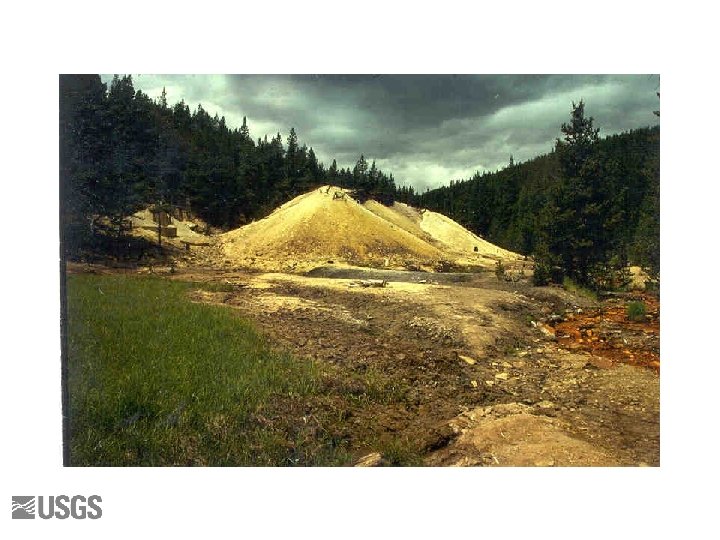
Acid Mine Drainage 147

Sulfide Oxidation • Pyrite/Marcasite are most important reactants • Need Pyrite, Oxygen, Water, and bugs • Oxidation of pyrite and formation of ferric hydroxide complexes and minerals generates acidic conditions

Iron Mountain, California • • Sulfide deposits at the top of a mountain Lots of precipitation Unsaturated conditions Tunnels drain

Picher, Oklahoma • • Flat topography Mines 200 to 500 ft below land surface Saturated after dewatering ceased Cut off the supply of oxygen

Simplified Reactions High p. H Fe. S 2 + 15/4 O 2 + 4 HCO 3 - = Fe(OH)3 + 2 SO 4 -2 + 4 CO 2 + 1/2 H 2 O Or Fe. S 2 + 15/4 O 2 + 7/2 H 2 O = Fe(OH)3 + 2 SO 4 -2 + 4 H+ Low p. H Fe. S 2 + 15/4 O 2 + 1/2 H 2 O = Fe+3 + SO 4 -2 + HSO 4 -

Additional reactions • Hydrous ferric oxides – Ferrihydrite – Goethite – Jarosite • Aluminum hydroxides – Alunite • Carbonates • Gypsum

Modeling Pyrite Oxidation Fe. S 2 + 15/4 O 2 + 7/2 H 2 O = Fe(OH)3 + 2 SO 4 -2 + 4 H+ • Pick the irreversible reactant: O 2 or Fe. S 2 – Oxygen rich environment of a tailings pile – We are going to react up to 50 mmol Fe. S 2 • Equilibrium reactions

REACTION 18. Exercise 1. React the pure water with 10 mmol of pyrite, maintaining equilibrium with atmosphreric oxygen. 2. React the pure water with 10 mmol of mackinawite, maintaining equilibrium with atmosphreric oxygen. 3. React the pure water with 10 mmol of sphalerite, maintaining equilibrium with atmosphreric oxygen.

REACTION 18. Questions 1. Write qualitative reactions that explain the p. H of the 3 solutions. 2. What p. H buffer starts to operate at p. Hs below 3? 3. Run the input file with wateq 4 f. database. What minerals may precipitate during pyrite oxidation?

Reaction 18. Answers 1. Question 1 Pyrite oxidation: Fe. S 2 + x. O 2 + y. H 2 O -> Fe+3 + 2 SO 4 -2 + H+ In addition, ferric iron hydrolizes to make additional H+: Fe+3 + H 2 O = Fe. OH+2 + H+ With net acid production to give p. H 2. Mackinawite oxidation: Fe. S + 2. 25 O 2 + H+ -> Fe+3 + SO 4 -2 +. 5 H 2 O But ferric iron hydrolizes Fe+3 + H 2 O = Fe. OH+2 + H+ With a net acid production that give p. H 4. Sphalerite oxidation: Zn. S + 2 O 2 -> Zn+2 + SO 4 -2 Zinc hydrolosis is minimal Zn+2 + H 2 O = Fe. OH+ + H+ Net result is p. H 7. 2. HSO 4 -/SO 4 -2 3. Iron oxyhydroxides, goethite (and often Fe(OH)3(a)) and jarosite. There is also a potassium jarosite and other solid solutions of jarosites. Aluminum has analogous minerals named alunite.

REACTION 20. Extra Credit Exercise 1. React the pure water with 20 mmol of pyrite, maintaining equilibrium with atmospheric oxygen and goethite. 2. Acid mine drainage is usually treated with limestone. Use the results of part 1 and equilibrate with O 2, goethite, and calcite.

REACTION 20. Questions 1. Write a net reaction for the PHREEQC results for the low-p. H simulation. 2. What are the p. H values with and without calcite equilibrium. 3. Looking at the results of the calciteequilibrated simulation, what additional reactions should be considered?

Reaction 20. Answers 1. 20 Fe. S 2 + 75 O 2 = 19 Fe. OOH +. 8 Fe(+3) + 27 HSO 4 - + 12 SO 4 -2 + 50 H+ 2. p. Hs are 1. 4 and 5. 8 without and with calcite equilibrium 3. Gypsum is supersaturated, and probably would precipitate. p. CO 2 is 1 atmosphere. If O 2 reacts to equilibrium with the atmosphere, logically, CO 2 would also.

Picher Oklahoma Abandoned Pb/Zn Mine mg/L • Mines are suboxic • Carbonates are present • Iron oxidizes in stream

Pyrite Oxidation Requires Pyrite/Marcasite O 2 H 2 O Bacteria Produces Ferrihydrite/Goethite, jarosite, alunite Gypsum if calcite is available Evaporites Possibly siderite Acid generation Pyrite > Fe. S > Zn. S

SOLID_SOLUTIONS—Composition of one or more solid solutions Trace elements and isotopes • List of solid solutions • Components of each solid solution Example SOLID_SOLUTION 21: Calcite solid solution Ca[13 C]O 3 Ca. CO 3 163

GAS_PHASE—Finite gas phase in equilibrium with solution • Gas bubbles that grow • Gas bubbles that fill a finite volume 164

GAS_PHASE—Composition of the gas phase Fixed volume or Fixed pressure • Initial volume • Initial pressure • Temperature • Partial pressure of each gas Example GAS_PHASE 1: Fixed pressure CO 2(g) 0. 0 CH 4(g) 0. 0 165