MOMENT GENERATING FUNCTION AND STATISTICAL DISTRIBUTIONS 1 MOMENT

MOMENT GENERATING FUNCTION AND STATISTICAL DISTRIBUTIONS 1

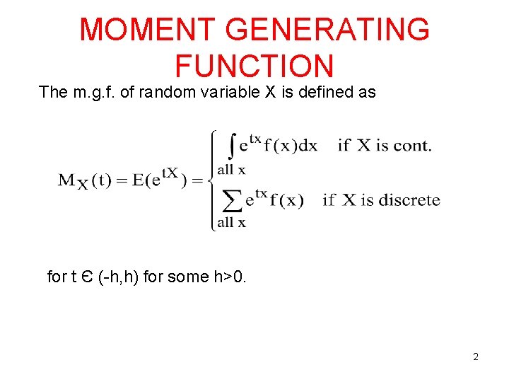
MOMENT GENERATING FUNCTION The m. g. f. of random variable X is defined as for t Є (-h, h) for some h>0. 2

Properties of m. g. f. • M(0)=E[1]=1 • If a r. v. X has m. g. f. M(t), then Y=a. X+b has a m. g. f. • • M. g. f does not always exists (e. g. Cauchy distribution) 3

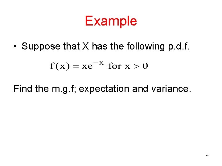
Example • Suppose that X has the following p. d. f. Find the m. g. f; expectation and variance. 4

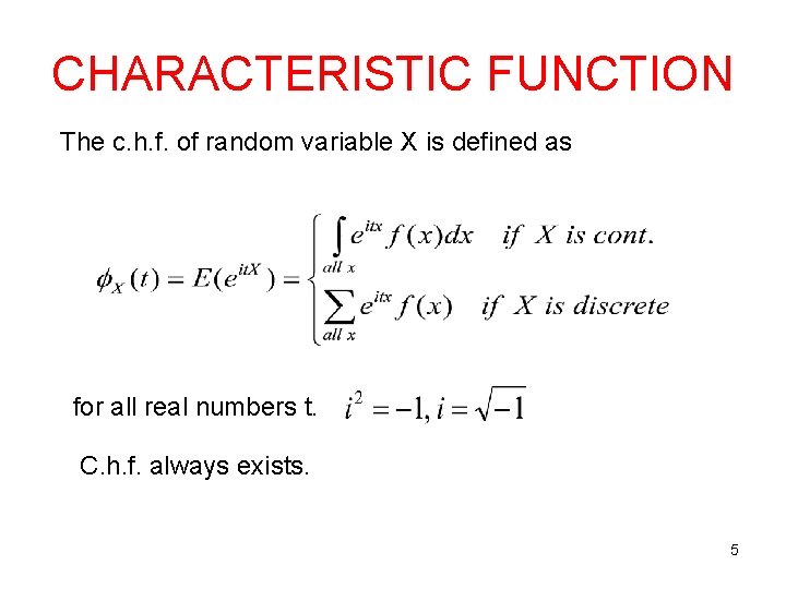
CHARACTERISTIC FUNCTION The c. h. f. of random variable X is defined as for all real numbers t. C. h. f. always exists. 5

Uniqueness Theorem: 1. If two r. v. s have mg. f. s that exist and are equal, then they have the same distribution. 2. If two r, v, s have the same distribution, then they have the same m. g. f. (if they exist) Similar statements are true for c. h. f. 6

STATISTICAL DISTRIBUTIONS 7

SOME DISCRETE PROBABILITY DISTRIBUTIONS Degenerate, Uniform, Bernoulli, Binomial, Poisson, Negative Binomial, Geometric, Hypergeometric 8

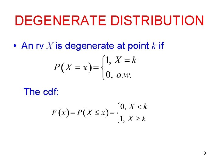
DEGENERATE DISTRIBUTION • An rv X is degenerate at point k if The cdf: 9

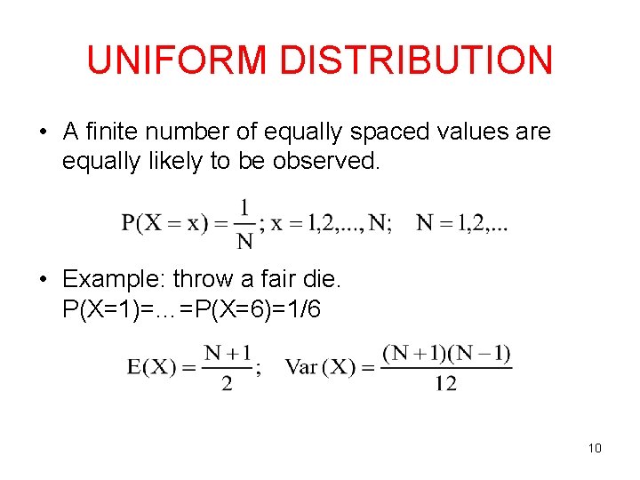
UNIFORM DISTRIBUTION • A finite number of equally spaced values are equally likely to be observed. • Example: throw a fair die. P(X=1)=…=P(X=6)=1/6 10

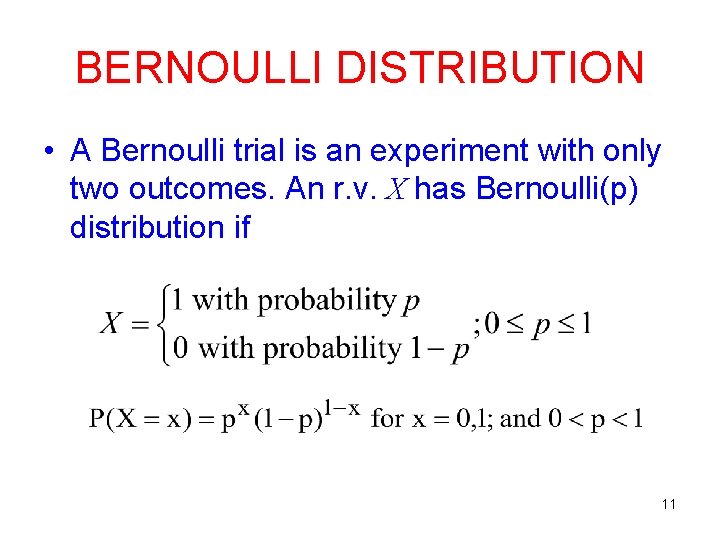
BERNOULLI DISTRIBUTION • A Bernoulli trial is an experiment with only two outcomes. An r. v. X has Bernoulli(p) distribution if 11

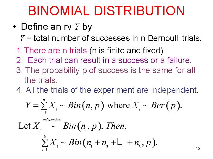
BINOMIAL DISTRIBUTION • Define an rv Y by Y = total number of successes in n Bernoulli trials. 1. There are n trials (n is finite and fixed). 2. Each trial can result in a success or a failure. 3. The probability p of success is the same for all the trials. 4. All the trials of the experiment are independent. 12

BINOMIAL DISTRIBUTION • Example: • There are black and white balls in a box. Select and record the color of the ball. Put it back and re-pick (sampling with replacement). • n: number of independent and identical trials • p: probability of success (e. g. probability of picking a black ball) • X: number of successes in n trials 13

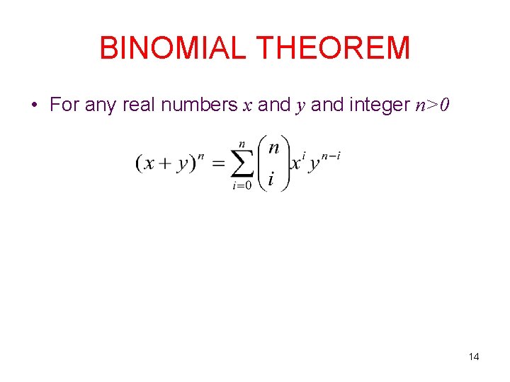
BINOMIAL THEOREM • For any real numbers x and y and integer n>0 14

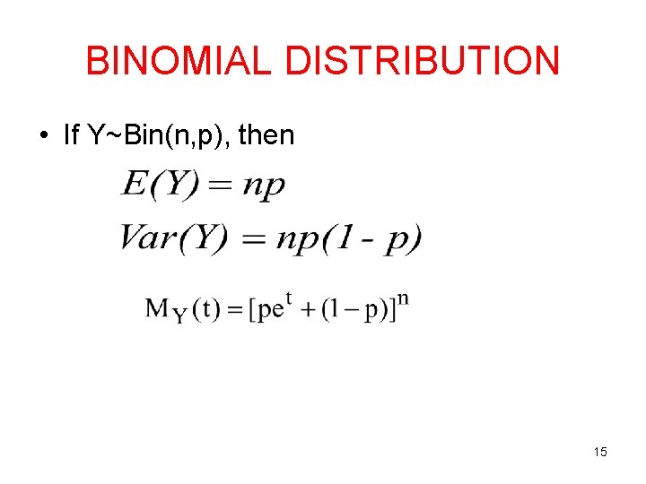
BINOMIAL DISTRIBUTION • If Y~Bin(n, p), then 15

POISSON DISTRIBUTION • The number of occurrences in a given time interval can be modeled by the Poisson distribution. • e. g. waiting for bus, waiting for customers to arrive in a bank. • Another application is in spatial distributions. • e. g. modeling the distribution of bomb hits in an area or the distribution of fish in a lake. 16

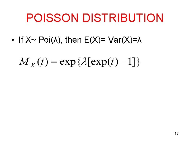
POISSON DISTRIBUTION • If X~ Poi(λ), then E(X)= Var(X)=λ 17

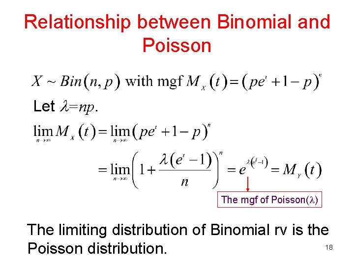
Relationship between Binomial and Poisson Let =np. The mgf of Poisson( ) The limiting distribution of Binomial rv is the 18 Poisson distribution.

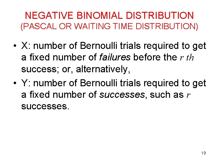
NEGATIVE BINOMIAL DISTRIBUTION (PASCAL OR WAITING TIME DISTRIBUTION) • X: number of Bernoulli trials required to get a fixed number of failures before the r th success; or, alternatively, • Y: number of Bernoulli trials required to get a fixed number of successes, such as r successes. 19

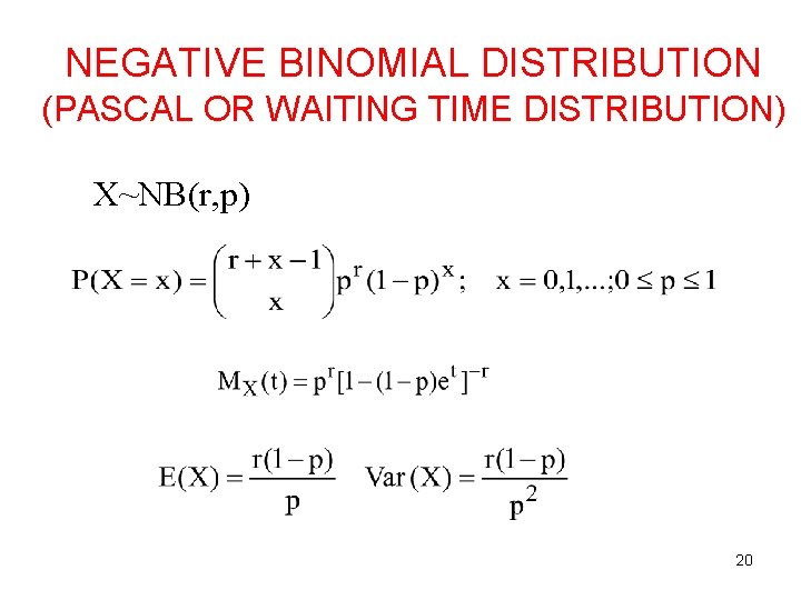
NEGATIVE BINOMIAL DISTRIBUTION (PASCAL OR WAITING TIME DISTRIBUTION) X~NB(r, p) 20

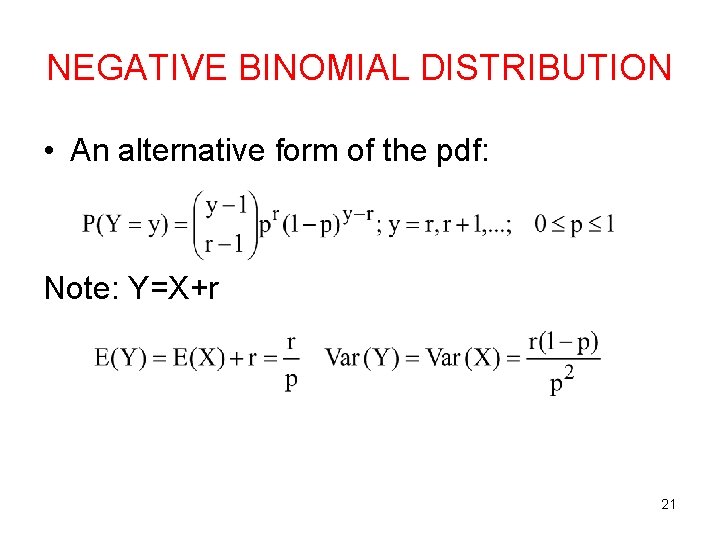
NEGATIVE BINOMIAL DISTRIBUTION • An alternative form of the pdf: Note: Y=X+r 21

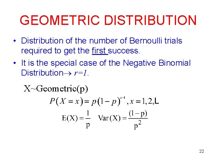
GEOMETRIC DISTRIBUTION • Distribution of the number of Bernoulli trials required to get the first success. • It is the special case of the Negative Binomial Distribution r=1. X~Geometric(p) 22

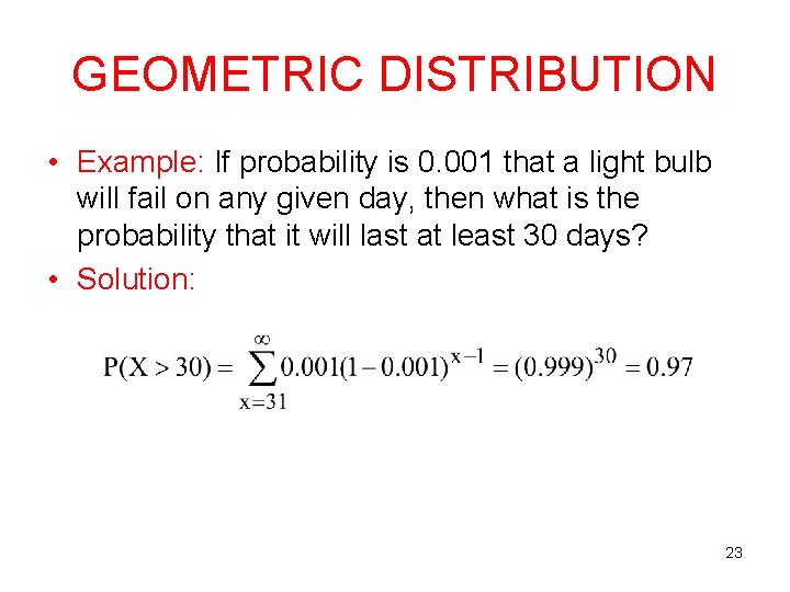
GEOMETRIC DISTRIBUTION • Example: If probability is 0. 001 that a light bulb will fail on any given day, then what is the probability that it will last at least 30 days? • Solution: 23

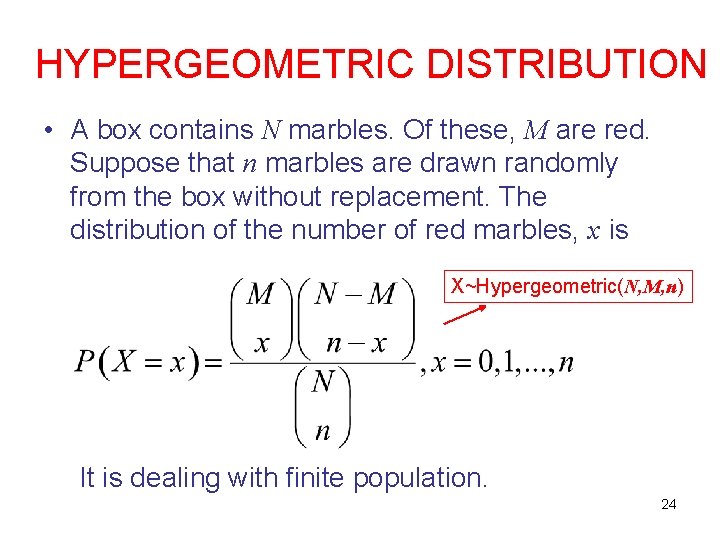
HYPERGEOMETRIC DISTRIBUTION • A box contains N marbles. Of these, M are red. Suppose that n marbles are drawn randomly from the box without replacement. The distribution of the number of red marbles, x is X~Hypergeometric(N, M, n) It is dealing with finite population. 24

SOME CONTINUOUS PROBABILITY DISTRIBUTIONS Uniform, Normal, Exponential, Gamma, Chi-Square, Beta Distributions 25

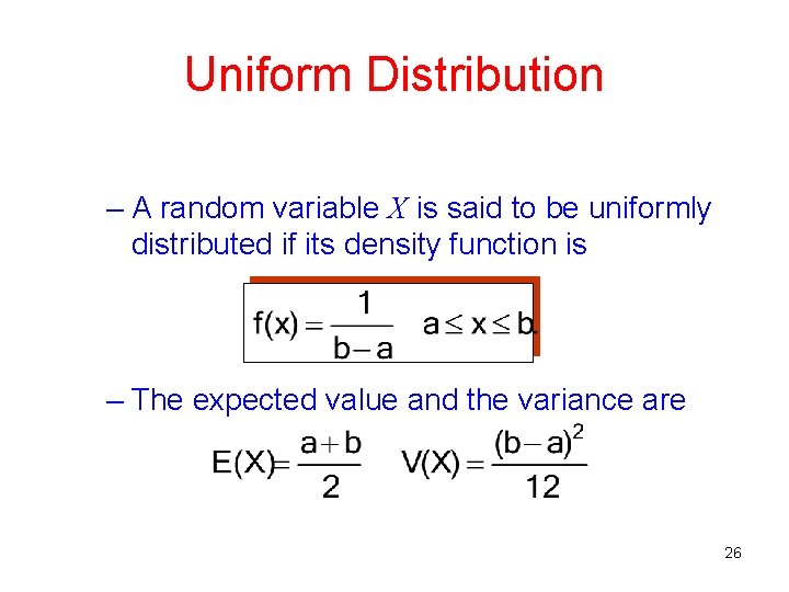
Uniform Distribution – A random variable X is said to be uniformly distributed if its density function is – The expected value and the variance are 26

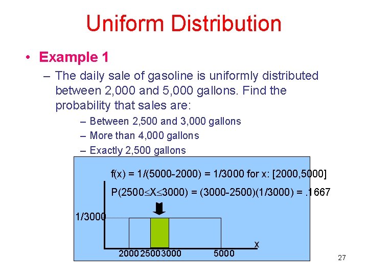
Uniform Distribution • Example 1 – The daily sale of gasoline is uniformly distributed between 2, 000 and 5, 000 gallons. Find the probability that sales are: – Between 2, 500 and 3, 000 gallons – More than 4, 000 gallons – Exactly 2, 500 gallons f(x) = 1/(5000 -2000) = 1/3000 for x: [2000, 5000] P(2500 X 3000) = (3000 -2500)(1/3000) =. 1667 1/3000 25003000 5000 x 27

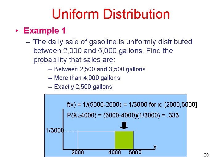
Uniform Distribution • Example 1 – The daily sale of gasoline is uniformly distributed between 2, 000 and 5, 000 gallons. Find the probability that sales are: – Between 2, 500 and 3, 500 gallons – More than 4, 000 gallons – Exactly 2, 500 gallons f(x) = 1/(5000 -2000) = 1/3000 for x: [2000, 5000] P(X 4000) = (5000 -4000)(1/3000) =. 333 1/3000 2000 4000 5000 x 28

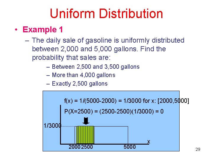
Uniform Distribution • Example 1 – The daily sale of gasoline is uniformly distributed between 2, 000 and 5, 000 gallons. Find the probability that sales are: – Between 2, 500 and 3, 500 gallons – More than 4, 000 gallons – Exactly 2, 500 gallons f(x) = 1/(5000 -2000) = 1/3000 for x: [2000, 5000] P(X=2500) = (2500 -2500)(1/3000) = 0 1/3000 2500 5000 x 29

Normal Distribution • This is the most popular continuous distribution. – Many distributions can be approximated by a normal distribution. – The normal distribution is the cornerstone distribution of statistical inference. 30

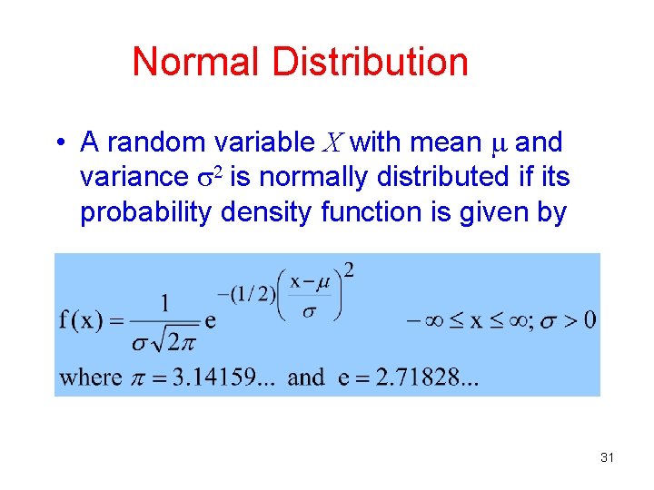
Normal Distribution • A random variable X with mean and variance 2 is normally distributed if its probability density function is given by 31

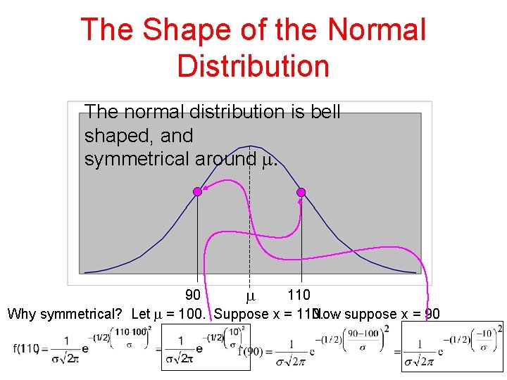
The Shape of the Normal Distribution The normal distribution is bell shaped, and symmetrical around . 90 110 Why symmetrical? Let = 100. Suppose x = 110. Now suppose x = 90

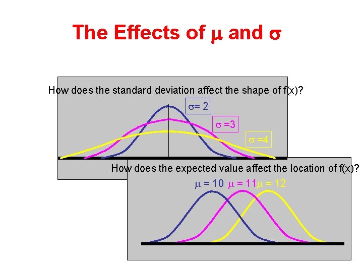
The Effects of m and s How does the standard deviation affect the shape of f(x)? = 2 =3 =4 How does the expected value affect the location of f(x)? = 10 = 11 = 12 33

Finding Normal Probabilities • Two facts help calculate normal probabilities: – The normal distribution is symmetrical. – Any normal distribution can be transformed into a specific normal distribution called… “STANDARD NORMAL DISTRIBUTION” Example The amount of time it takes to assemble a computer is normally distributed, with a mean of 50 minutes and a standard deviation of 10 minutes. What is the probability that a computer is assembled in a time between 45 and 60 minutes? 34

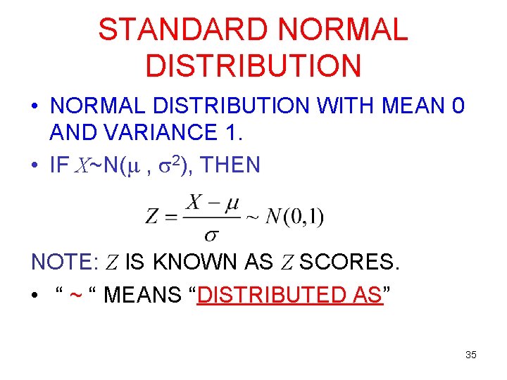
STANDARD NORMAL DISTRIBUTION • NORMAL DISTRIBUTION WITH MEAN 0 AND VARIANCE 1. • IF X~N( , 2), THEN NOTE: Z IS KNOWN AS Z SCORES. • “ ~ “ MEANS “DISTRIBUTED AS” 35

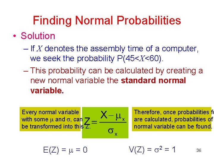
Finding Normal Probabilities • Solution – If X denotes the assembly time of a computer, we seek the probability P(45<X<60). – This probability can be calculated by creating a new normal variable the standard normal variable. Every normal variable with some and , can be transformed into this Z. E(Z) = = 0 Therefore, once probabilities fo are calculated, probabilities of normal variable can be found. V(Z) = 2 = 1 36

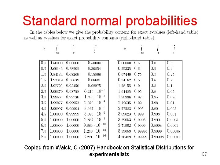
Standard normal probabilities Copied from Walck, C (2007) Handbook on Statistical Distributions for experimentalists 37

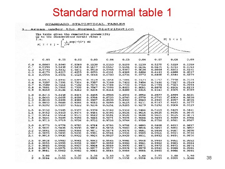
Standard normal table 1 38

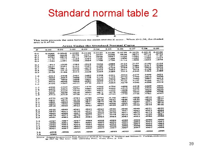
Standard normal table 2 39

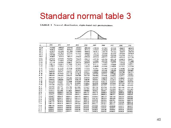
Standard normal table 3 40

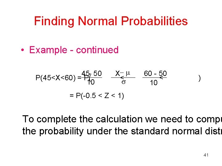
Finding Normal Probabilities • Example - continued 45 - 50 P(45<X<60) = P( 10 X < 60 - 50 < 10 ) = P(-0. 5 < Z < 1) To complete the calculation we need to compu the probability under the standard normal distr 41

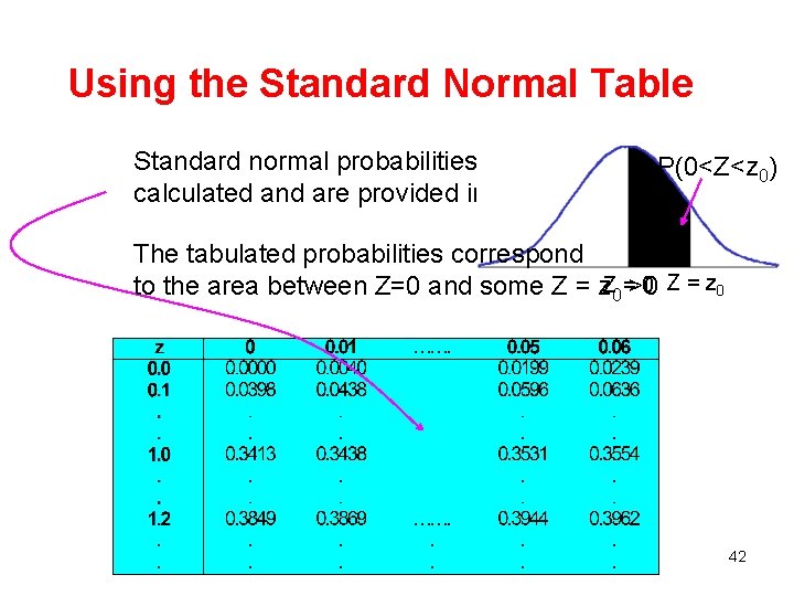
Using the Standard Normal Table Standard normal probabilities have been calculated and are provided in a table. P(0<Z<z 0) The tabulated probabilities correspond 0 Z = z 0 to the area between Z=0 and some Z = z. Z 0 =>0 42

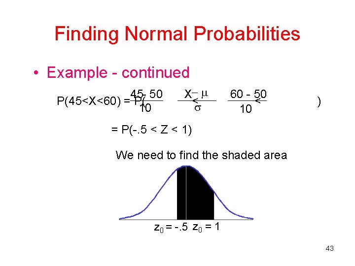
Finding Normal Probabilities • Example - continued 45 - 50 P(45<X<60) = P( 10 X < 60 - 50 < 10 ) = P(-. 5 < Z < 1) We need to find the shaded area z 0 = -. 5 z 0 = 1 43

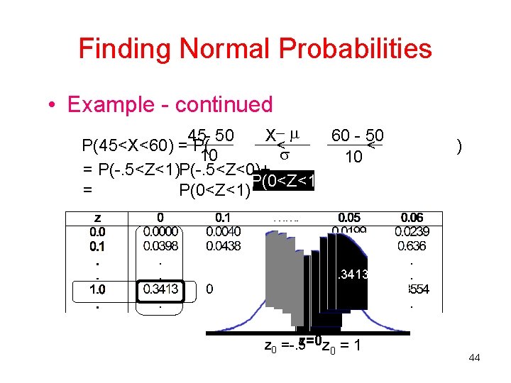
Finding Normal Probabilities • Example - continued 45 - 50 X 60 - 50 P(45<X<60) = P( < < 10 10 = P(-. 5<Z<1)P(-. 5<Z<0)+ P(0<Z<1 = P(0<Z<1) ) . 3413 z=0 z = 1 z 0 =-. 5 0 44

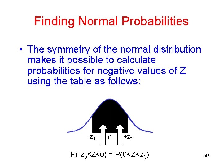
Finding Normal Probabilities • The symmetry of the normal distribution makes it possible to calculate probabilities for negative values of Z using the table as follows: -z 0 0 +z 0 P(-z 0<Z<0) = P(0<Z<z 0) 45

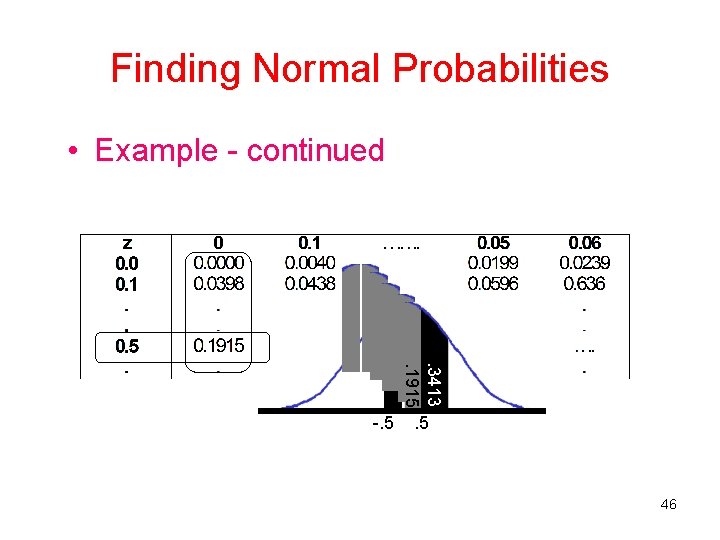
Finding Normal Probabilities • Example - continued . 3413. 1915 -. 5 46

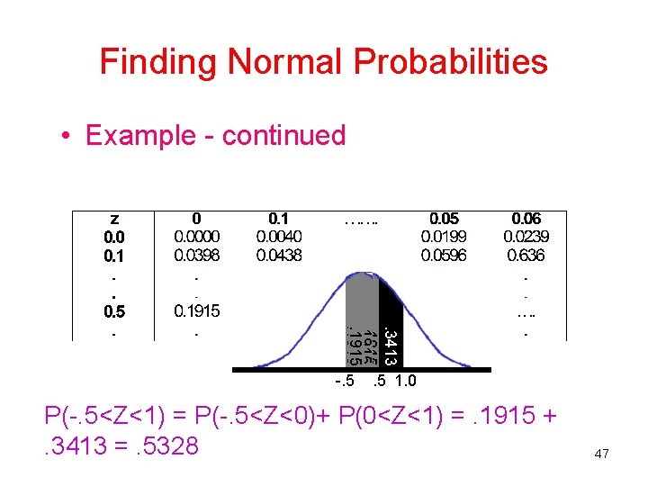
Finding Normal Probabilities • Example - continued . 3413. 1915 -. 5 1. 0 P(-. 5<Z<1) = P(-. 5<Z<0)+ P(0<Z<1) =. 1915 +. 3413 =. 5328 47

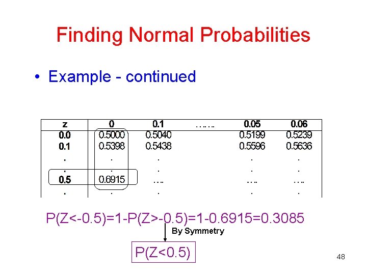
Finding Normal Probabilities • Example - continued . 3413 P(Z<-0. 5)=1 -P(Z>-0. 5)=1 -0. 6915=0. 3085 By Symmetry P(Z<0. 5) 48

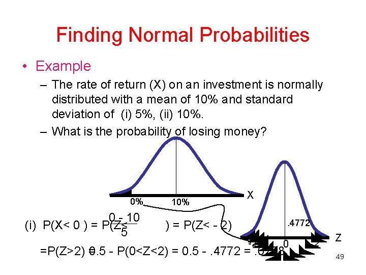
Finding Normal Probabilities • Example – The rate of return (X) on an investment is normally distributed with a mean of 10% and standard deviation of (i) 5%, (ii) 10%. – What is the probability of losing money? 0% 0 - 10 (i) P(X< 0 ) = P(Z< 5 10% X. 4772 ) = P(Z< - 2) -2 0 =P(Z>2) = 0. 5 - P(0<Z<2) = 0. 5 -. 4772 =. 0228 2 Z 49

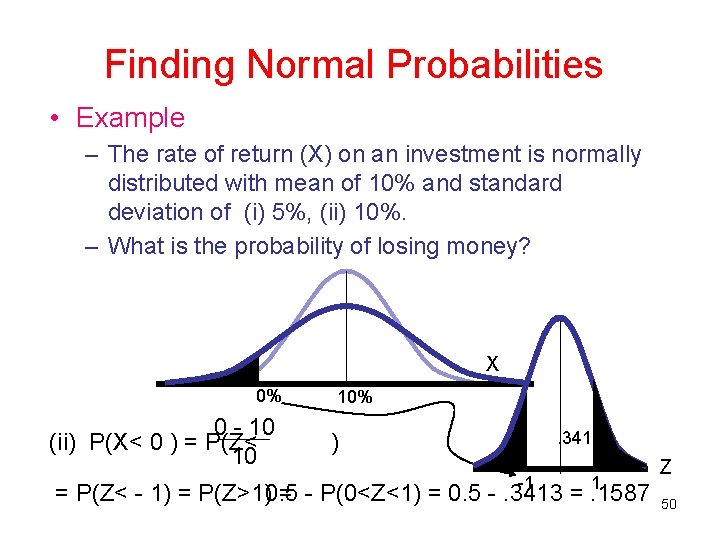
Finding Normal Probabilities • Example – The rate of return (X) on an investment is normally distributed with mean of 10% and standard deviation of (i) 5%, (ii) 10%. – What is the probability of losing money? X 0% 0 - 10 (ii) P(X< 0 ) = P(Z< 10 10%. 3413 ) -1 1 = P(Z< - 1) = P(Z>1)0. 5 = - P(0<Z<1) = 0. 5 -. 3413 =. 1587 Z 50

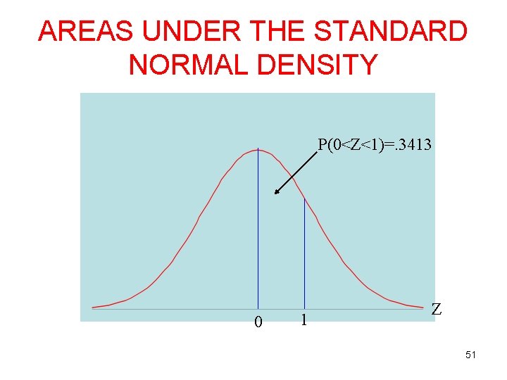
AREAS UNDER THE STANDARD NORMAL DENSITY P(0<Z<1)=. 3413 0 1 Z 51

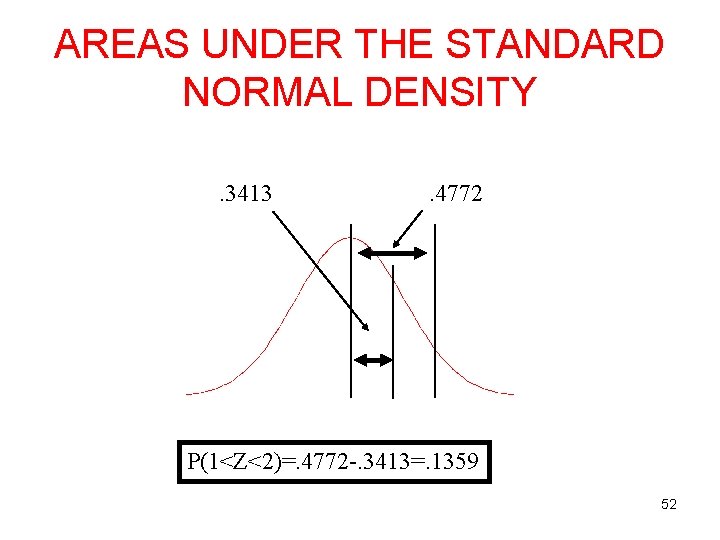
AREAS UNDER THE STANDARD NORMAL DENSITY. 3413 . 4772 P(1<Z<2)=. 4772 -. 3413=. 1359 52

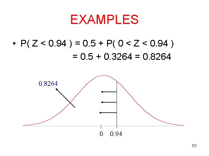
EXAMPLES • P( Z < 0. 94 ) = 0. 5 + P( 0 < Z < 0. 94 ) = 0. 5 + 0. 3264 = 0. 8264 0 0. 94 53

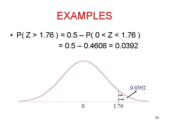
EXAMPLES • P( Z > 1. 76 ) = 0. 5 – P( 0 < Z < 1. 76 ) = 0. 5 – 0. 4608 = 0. 0392 0 1. 76 54

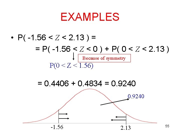
EXAMPLES • P( -1. 56 < Z < 2. 13 ) = = P( -1. 56 < Z < 0 ) + P( 0 < Z < 2. 13 ) Because of symmetry P(0 < Z < 1. 56) = 0. 4406 + 0. 4834 = 0. 9240 -1. 56 2. 13 55

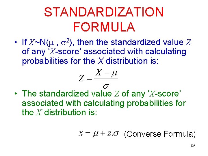
STANDARDIZATION FORMULA • If X~N( , 2), then the standardized value Z of any ‘X-score’ associated with calculating probabilities for the X distribution is: • The standardized value Z of any ‘X-score’ associated with calculating probabilities for the X distribution is: (Converse Formula) 56

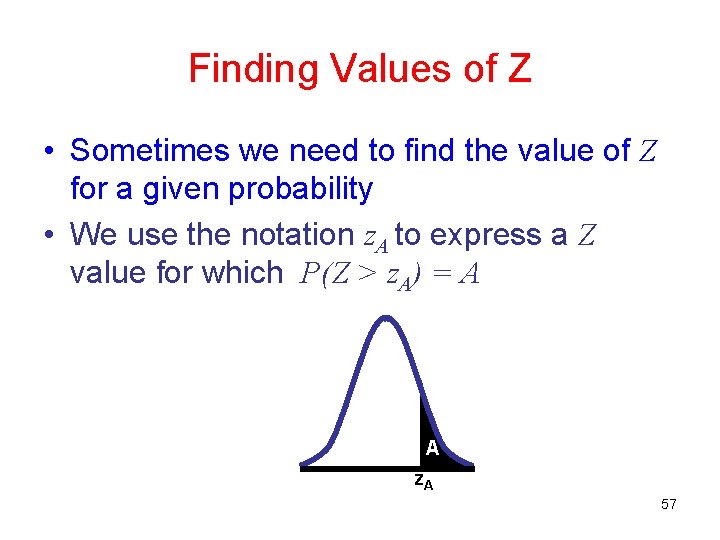
Finding Values of Z • Sometimes we need to find the value of Z for a given probability • We use the notation z. A to express a Z value for which P(Z > z. A) = A A z. A 57

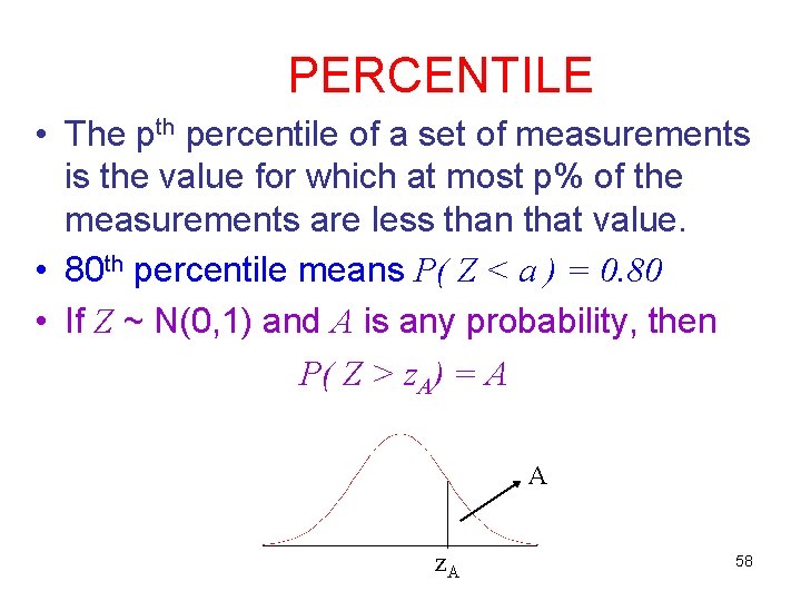
PERCENTILE • The pth percentile of a set of measurements is the value for which at most p% of the measurements are less than that value. • 80 th percentile means P( Z < a ) = 0. 80 • If Z ~ N(0, 1) and A is any probability, then P( Z > z. A) = A A z. A 58

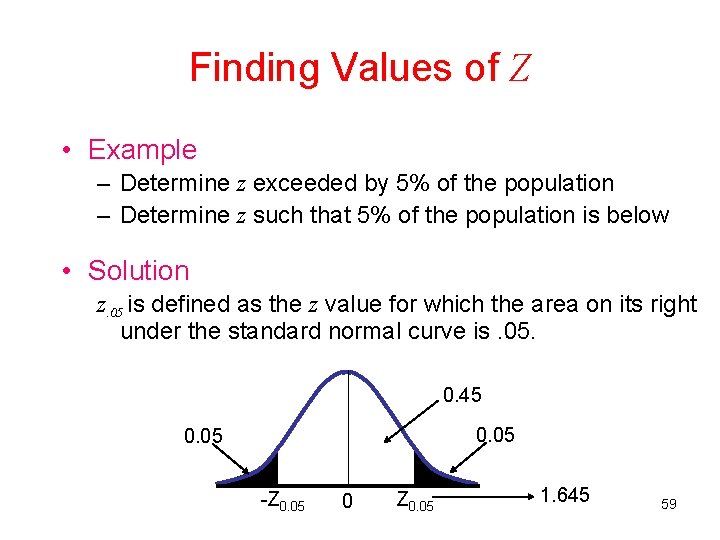
Finding Values of Z • Example – Determine z exceeded by 5% of the population – Determine z such that 5% of the population is below • Solution z. 05 is defined as the z value for which the area on its right under the standard normal curve is. 05. 0. 45 0. 05 -Z 0. 05 0 Z 0. 05 1. 645 59

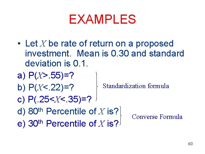
EXAMPLES • Let X be rate of return on a proposed investment. Mean is 0. 30 and standard deviation is 0. 1. a) P(X>. 55)=? Standardization formula b) P(X<. 22)=? c) P(. 25<X<. 35)=? d) 80 th Percentile of X is? Converse Formula e) 30 th Percentile of X is? 60

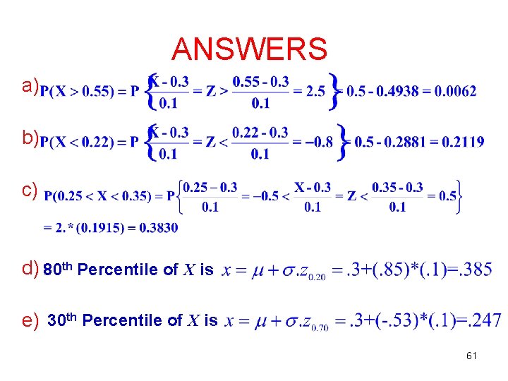
ANSWERS a) b) c) d) 80 th Percentile of X is e) 30 th Percentile of X is 61

The Normal Approximation to the Binomial Distribution • The normal distribution provides a close approximation to the Binomial distribution when n (number of trials) is large and p (success probability) is close to 0. 5. • The approximation is used only when np 5 and n(1 -p) 5 62

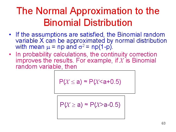
The Normal Approximation to the Binomial Distribution • If the assumptions are satisfied, the Binomial random variable X can be approximated by normal distribution with mean = np and 2 = np(1 -p). • In probability calculations, the continuity correction improves the results. For example, if X is Binomial random variable, then P(X a) ≈ P(X<a+0. 5) P(X a) ≈ P(X>a-0. 5) 63

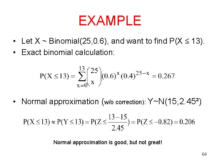
EXAMPLE • Let X ~ Binomial(25, 0. 6), and want to find P(X ≤ 13). • Exact binomial calculation: • Normal approximation (w/o correction): Y~N(15, 2. 45²) Normal approximation is good, but not great! 64

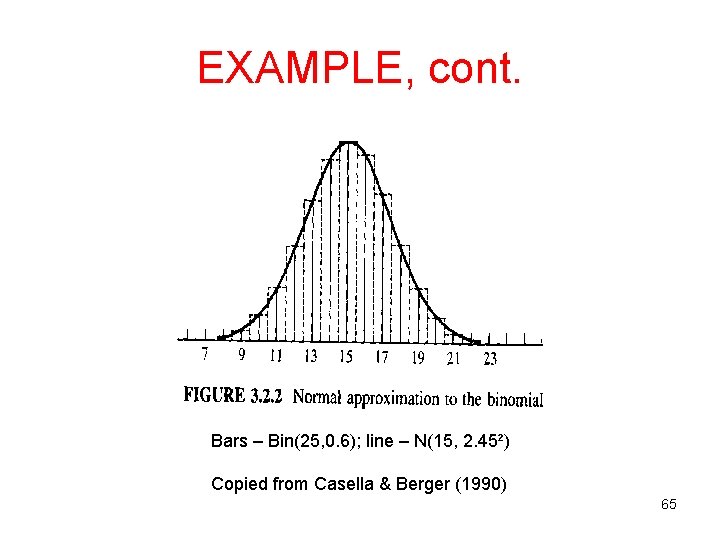
EXAMPLE, cont. Bars – Bin(25, 0. 6); line – N(15, 2. 45²) Copied from Casella & Berger (1990) 65

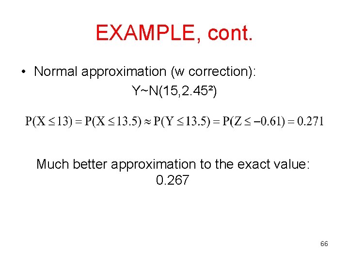
EXAMPLE, cont. • Normal approximation (w correction): Y~N(15, 2. 45²) Much better approximation to the exact value: 0. 267 66

Exponential Distribution • The exponential distribution can be used to model – the length of time between telephone calls – the length of time between arrivals at a service station – the lifetime of electronic components. • When the number of occurrences of an event follows the Poisson distribution, the time between occurrences follows the exponential distribution. 67

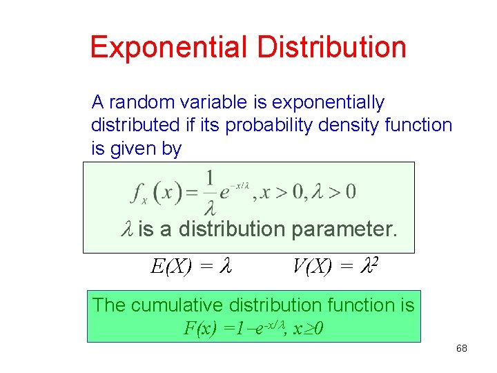
Exponential Distribution A random variable is exponentially distributed if its probability density function is given by f(x) = e- x, x>=0. is a distribution parameter. is the distribution parameter >0). E(X) = V(X) = 2 The cumulative distribution function is F(x) =1 e-x/ , x 0 68

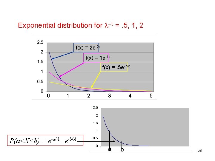
Exponential distribution for 1 =. 5, 1, 2 f(x) = 2 e-2 x f(x) = 1 e-1 x f(x) =. 5 e-. 5 x 0 1 2 3 4 5 P(a<X<b) = e-a/ e-b/ a b 69

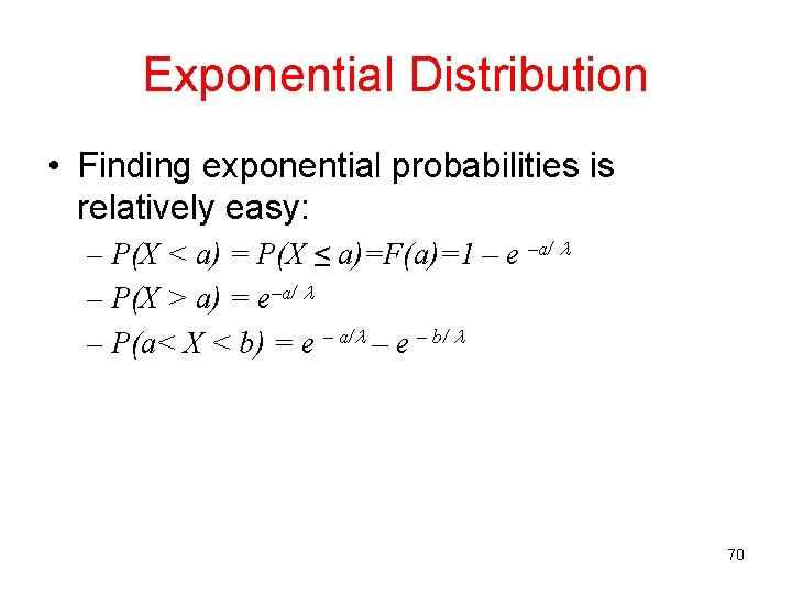
Exponential Distribution • Finding exponential probabilities is relatively easy: – P(X < a) = P(X ≤ a)=F(a)=1 – e –a/ – P(X > a) = e–a/ – P(a< X < b) = e – a/ – e – b/ 70

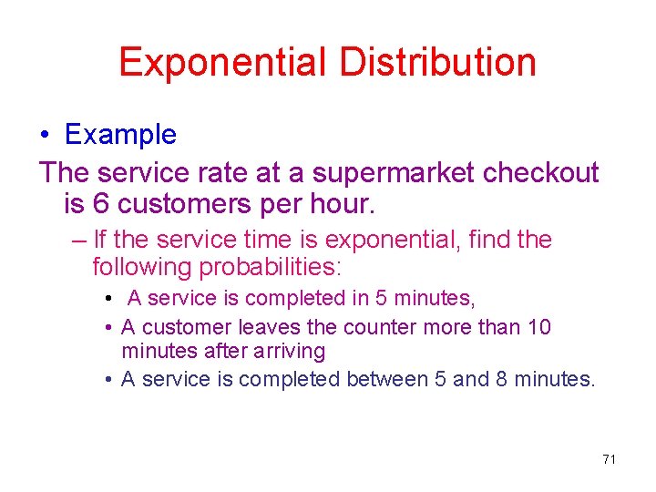
Exponential Distribution • Example The service rate at a supermarket checkout is 6 customers per hour. – If the service time is exponential, find the following probabilities: • A service is completed in 5 minutes, • A customer leaves the counter more than 10 minutes after arriving • A service is completed between 5 and 8 minutes. 71

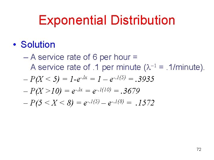
Exponential Distribution • Solution – A service rate of 6 per hour = A service rate of. 1 per minute ( 1 =. 1/minute). – P(X < 5) = 1 -e-. lx = 1 – e-. 1(5) =. 3935 – P(X >10) = e-. lx = e-. 1(10) =. 3679 – P(5 < X < 8) = e-. 1(5) – e-. 1(8) =. 1572 72

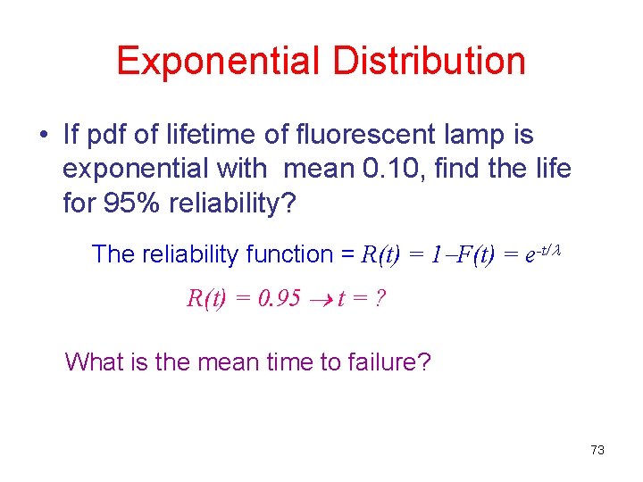
Exponential Distribution • If pdf of lifetime of fluorescent lamp is exponential with mean 0. 10, find the life for 95% reliability? The reliability function = R(t) = 1 F(t) = e-t/ R(t) = 0. 95 t = ? What is the mean time to failure? 73

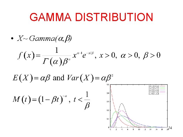
GAMMA DISTRIBUTION • X~ Gamma( , ) 74

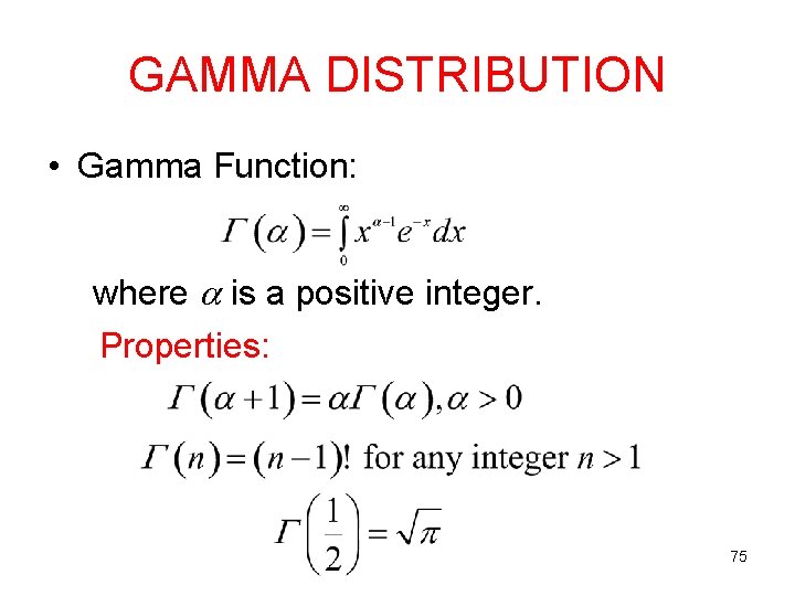
GAMMA DISTRIBUTION • Gamma Function: where is a positive integer. Properties: 75

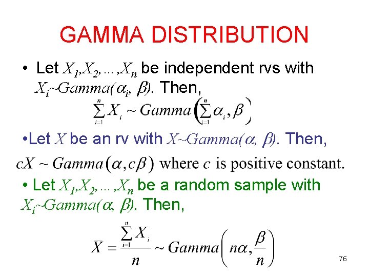
GAMMA DISTRIBUTION • Let X 1, X 2, …, Xn be independent rvs with Xi~Gamma( i, ). Then, • Let X be an rv with X~Gamma( , ). Then, • Let X 1, X 2, …, Xn be a random sample with Xi~Gamma( , ). Then, 76

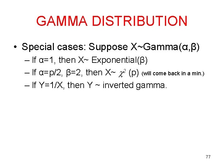
GAMMA DISTRIBUTION • Special cases: Suppose X~Gamma(α, β) – If α=1, then X~ Exponential(β) – If α=p/2, β=2, then X~ 2 (p) (will come back in a min. ) – If Y=1/X, then Y ~ inverted gamma. 77

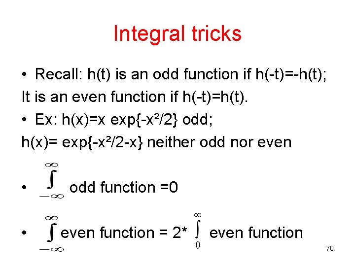
Integral tricks • Recall: h(t) is an odd function if h(-t)=-h(t); It is an even function if h(-t)=h(t). • Ex: h(x)=x exp{-x²/2} odd; h(x)= exp{-x²/2 -x} neither odd nor even • odd function =0 • even function = 2* even function 78

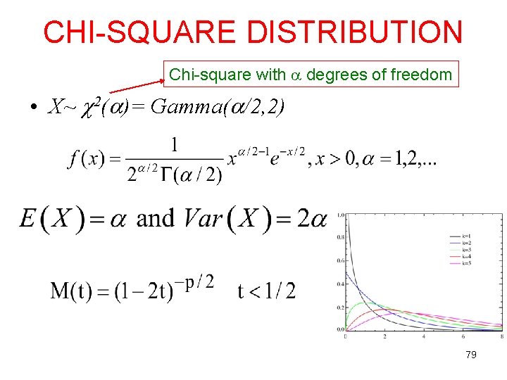
CHI-SQUARE DISTRIBUTION Chi-square with degrees of freedom • X~ 2( )= Gamma( /2, 2) 79

DEGREES OF FREEDOM • In statistics, the phrase degrees of freedom is used to describe the number of values in the final calculation of a statistic that are free to vary. • The number of independent pieces of information that go into the estimate of a parameter is called the degrees of freedom (df). • How many components need to be known before the vector is fully determined? 80

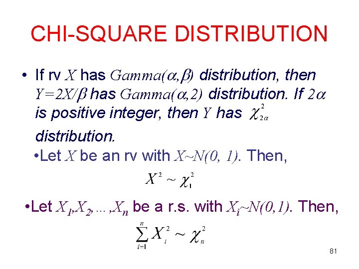
CHI-SQUARE DISTRIBUTION • If rv X has Gamma( , ) distribution, then Y=2 X/ has Gamma( , 2) distribution. If 2 is positive integer, then Y has distribution. • Let X be an rv with X~N(0, 1). Then, • Let X 1, X 2, …, Xn be a r. s. with Xi~N(0, 1). Then, 81

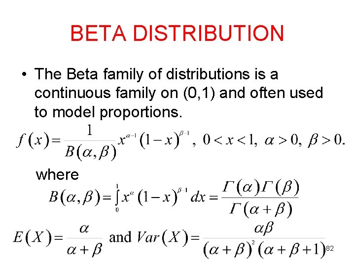
BETA DISTRIBUTION • The Beta family of distributions is a continuous family on (0, 1) and often used to model proportions. where 82

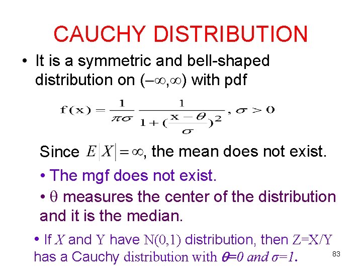
CAUCHY DISTRIBUTION • It is a symmetric and bell-shaped distribution on ( , ) with pdf , the mean does not exist. Since • The mgf does not exist. • measures the center of the distribution and it is the median. • If X and Y have N(0, 1) distribution, then Z=X/Y has a Cauchy distribution with =0 and σ=1. 83

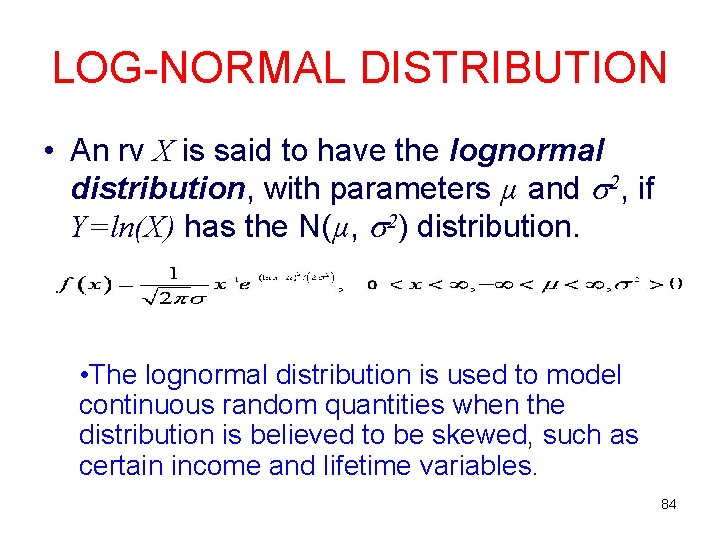
LOG-NORMAL DISTRIBUTION • An rv X is said to have the lognormal distribution, with parameters µ and 2, if Y=ln(X) has the N(µ, 2) distribution. • The lognormal distribution is used to model continuous random quantities when the distribution is believed to be skewed, such as certain income and lifetime variables. 84

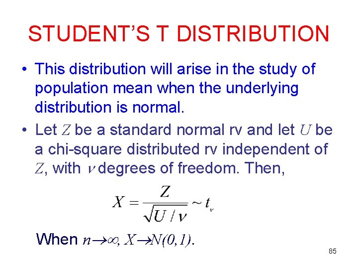
STUDENT’S T DISTRIBUTION • This distribution will arise in the study of population mean when the underlying distribution is normal. • Let Z be a standard normal rv and let U be a chi-square distributed rv independent of Z, with degrees of freedom. Then, When n , X N(0, 1). 85

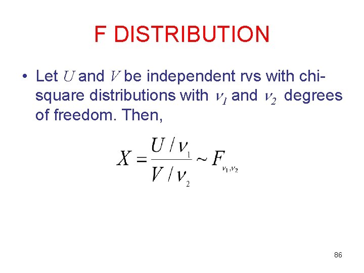
F DISTRIBUTION • Let U and V be independent rvs with chisquare distributions with 1 and 2 degrees of freedom. Then, 86

MULTIVARIATE DISTRIBUTIONS 87

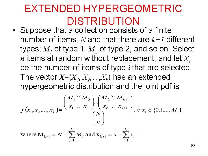
EXTENDED HYPERGEOMETRIC DISTRIBUTION • Suppose that a collection consists of a finite number of items, N and that there are k+1 different types; M 1 of type 1, M 2 of type 2, and so on. Select n items at random without replacement, and let Xi be the number of items of type i that are selected. The vector X=(X 1, X 2, …, Xk) has an extended hypergeometric distribution and the joint pdf is 88

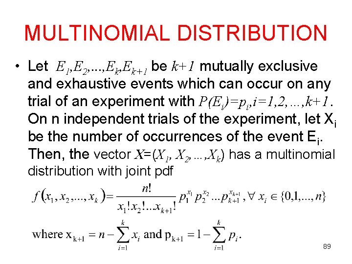
MULTINOMIAL DISTRIBUTION • Let E 1, E 2, . . . , Ek+1 be k+1 mutually exclusive and exhaustive events which can occur on any trial of an experiment with P(Ei)=pi, i=1, 2, …, k+1. On n independent trials of the experiment, let Xi be the number of occurrences of the event Ei. Then, the vector X=(X 1, X 2, …, Xk) has a multinomial distribution with joint pdf 89

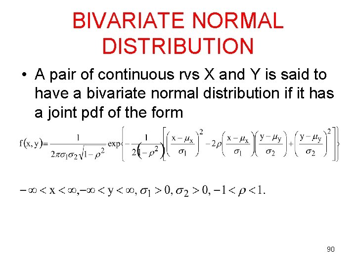
BIVARIATE NORMAL DISTRIBUTION • A pair of continuous rvs X and Y is said to have a bivariate normal distribution if it has a joint pdf of the form 90

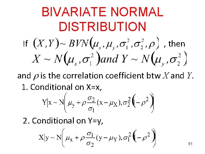
BIVARIATE NORMAL DISTRIBUTION If , then and is the correlation coefficient btw X and Y. 1. Conditional on X=x, 2. Conditional on Y=y, 91