Molecular Evolution Selection the ratio between the number

Molecular Evolution: Selection • the ratio between the number of nonsynonymous substitutions (KA) and synonymous substitutions (KS) in a gene during a specific evolutionary period. • Assuming that KS provides an index of the random mutation rate, the KA/KS ratio measures whether the rate of protein evolution differs from the rate expected under neutral drift. – If KA>KS, this is taken to indicate accelerated aminoacid change, which might be due to positive selection. – Conversely, if KA<KS, this suggests purifying selection.

Brain Development in Primates • MCPH 1 (the gene that encodes microcephalin) • and ASPM (abnormal-spindle-like, microcephaly associated) • Both MCPH 1 and ASPM are evolutionarily ancient, with orthologues that are likely to be present in all chordates

MCPH

MCPH

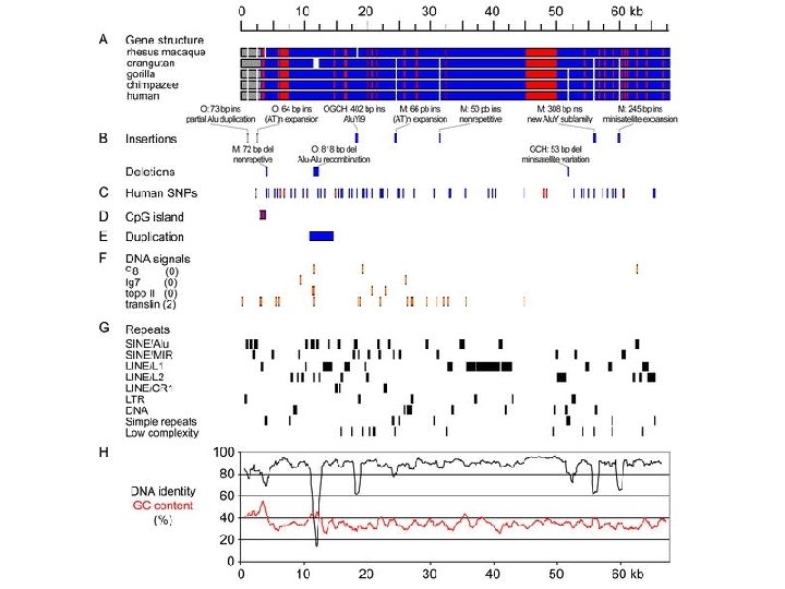
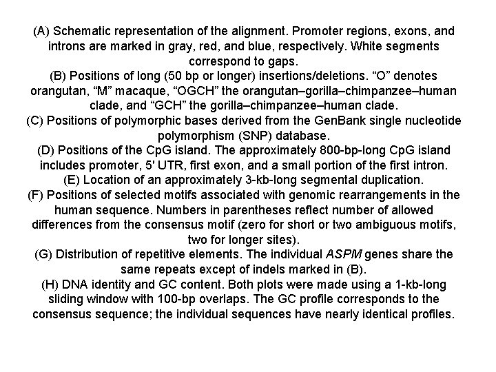
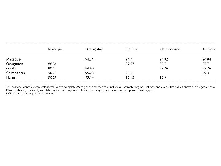
(A) Schematic representation of the alignment. Promoter regions, exons, and introns are marked in gray, red, and blue, respectively. White segments correspond to gaps. (B) Positions of long (50 bp or longer) insertions/deletions. “O” denotes orangutan, “M” macaque, “OGCH” the orangutan–gorilla–chimpanzee–human clade, and “GCH” the gorilla–chimpanzee–human clade. (C) Positions of polymorphic bases derived from the Gen. Bank single nucleotide polymorphism (SNP) database. (D) Positions of the Cp. G island. The approximately 800 -bp-long Cp. G island includes promoter, 5′ UTR, first exon, and a small portion of the first intron. (E) Location of an approximately 3 -kb-long segmental duplication. (F) Positions of selected motifs associated with genomic rearrangements in the human sequence. Numbers in parentheses reflect number of allowed differences from the consensus motif (zero for short or two ambiguous motifs, two for longer sites). (G) Distribution of repetitive elements. The individual ASPM genes share the same repeats except of indels marked in (B). (H) DNA identity and GC content. Both plots were made using a 1 -kb-long sliding window with 100 -bp overlaps. The GC profile corresponds to the consensus sequence; the individual sequences have nearly identical profiles.

Linkage Studies Monogenic and Complex Studies

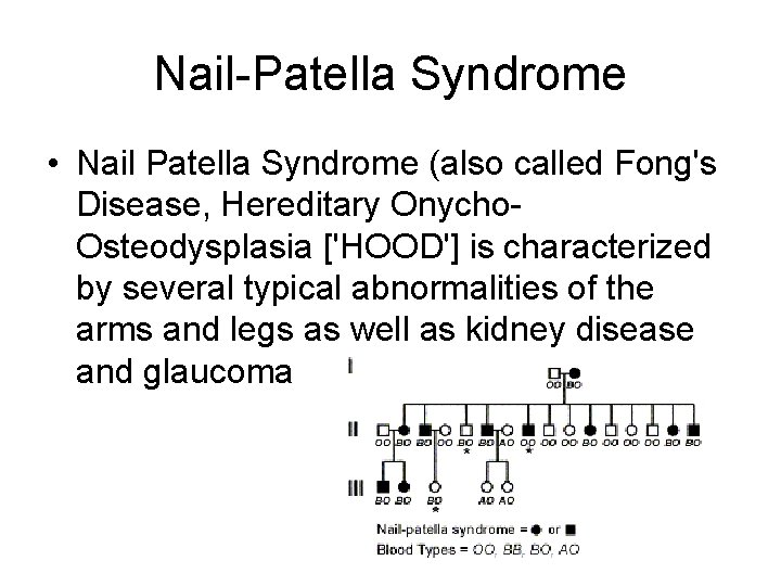
Nail-Patella Syndrome • Nail Patella Syndrome (also called Fong's Disease, Hereditary Onycho. Osteodysplasia ['HOOD'] is characterized by several typical abnormalities of the arms and legs as well as kidney disease and glaucoma

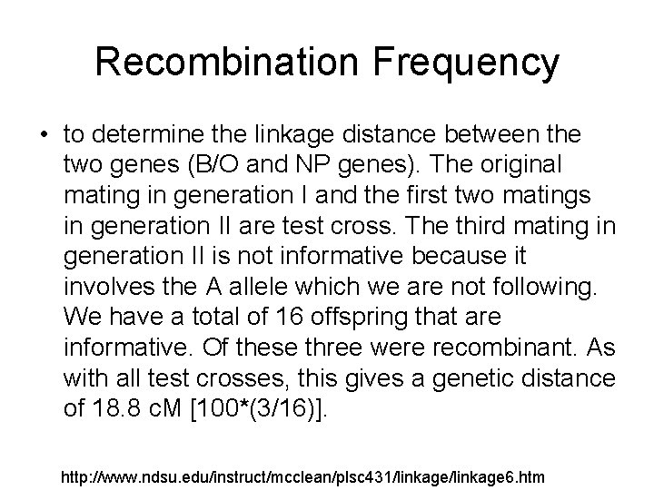
Recombination Frequency • to determine the linkage distance between the two genes (B/O and NP genes). The original mating in generation I and the first two matings in generation II are test cross. The third mating in generation II is not informative because it involves the A allele which we are not following. We have a total of 16 offspring that are informative. Of these three were recombinant. As with all test crosses, this gives a genetic distance of 18. 8 c. M [100*(3/16)]. http: //www. ndsu. edu/instruct/mcclean/plsc 431/linkage 6. htm

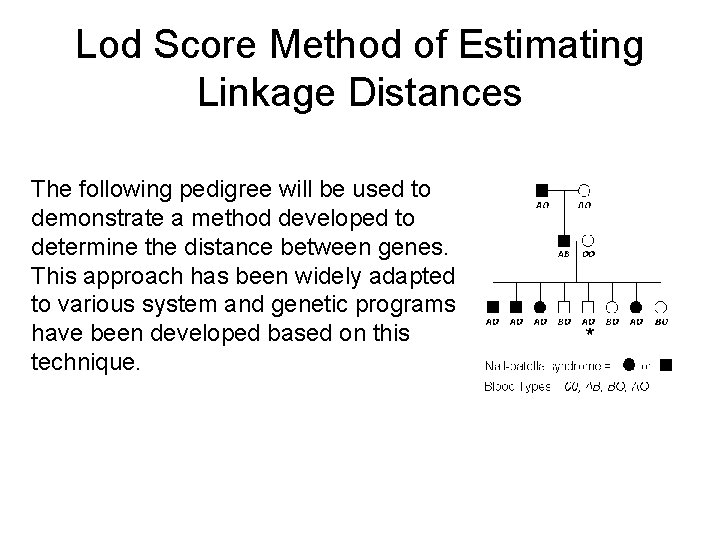
Lod Score Method of Estimating Linkage Distances The following pedigree will be used to demonstrate a method developed to determine the distance between genes. This approach has been widely adapted to various system and genetic programs have been developed based on this technique.

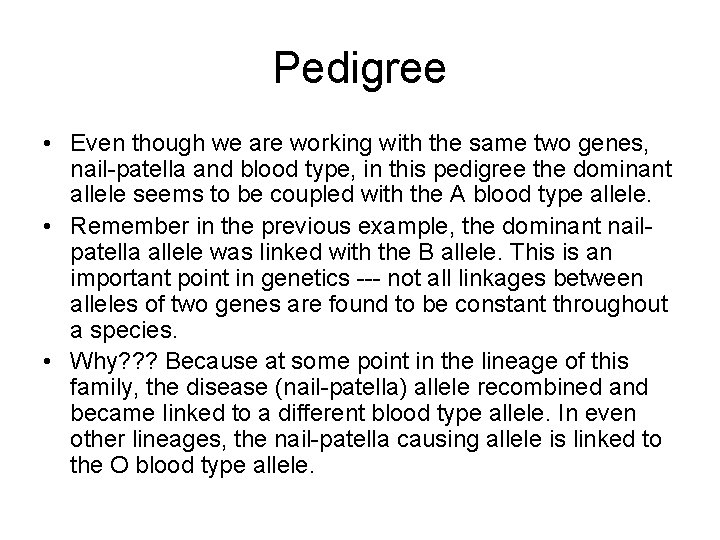
Pedigree • Even though we are working with the same two genes, nail-patella and blood type, in this pedigree the dominant allele seems to be coupled with the A blood type allele. • Remember in the previous example, the dominant nailpatella allele was linked with the B allele. This is an important point in genetics --- not all linkages between alleles of two genes are found to be constant throughout a species. • Why? ? ? Because at some point in the lineage of this family, the disease (nail-patella) allele recombined and became linked to a different blood type allele. In even other lineages, the nail-patella causing allele is linked to the O blood type allele.

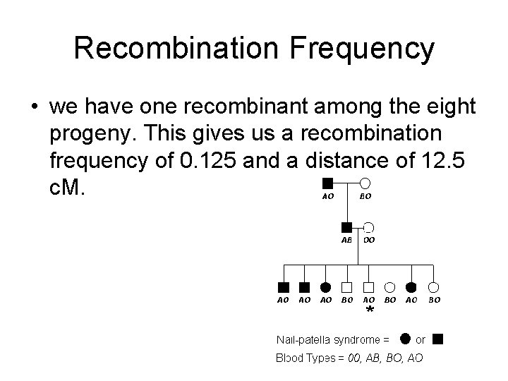
Recombination Frequency • we have one recombinant among the eight progeny. This gives us a recombination frequency of 0. 125 and a distance of 12. 5 c. M.

LOD Score Method • developed by Newton E. Morton, and is an iterative approach that include a series of lod scores calculated from a number of proposed linkage distance.

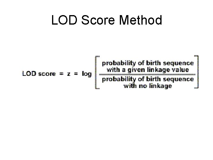
LOD Score Method • A linkage distance is estimated, and given that estimate, the probability of a given birth sequence is calculated. That value is then divided by the probability of a given birth sequence assuming that the genes are unlinked. The log of this value is calculated, and that value is the lod score for this linkage distance estimate.

LOD Score Method

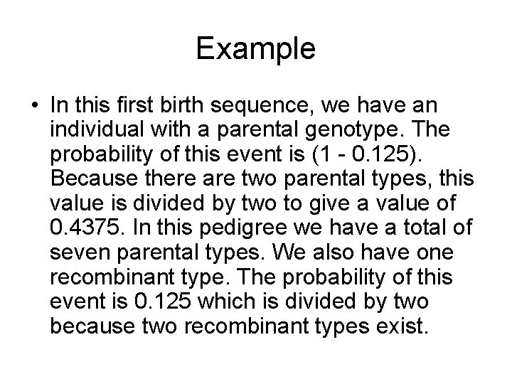
Example • In this first birth sequence, we have an individual with a parental genotype. The probability of this event is (1 - 0. 125). Because there are two parental types, this value is divided by two to give a value of 0. 4375. In this pedigree we have a total of seven parental types. We also have one recombinant type. The probability of this event is 0. 125 which is divided by two because two recombinant types exist.

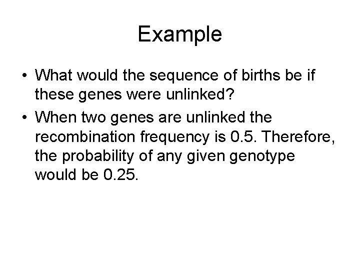
Example • What would the sequence of births be if these genes were unlinked? • When two genes are unlinked the recombination frequency is 0. 5. Therefore, the probability of any given genotype would be 0. 25.

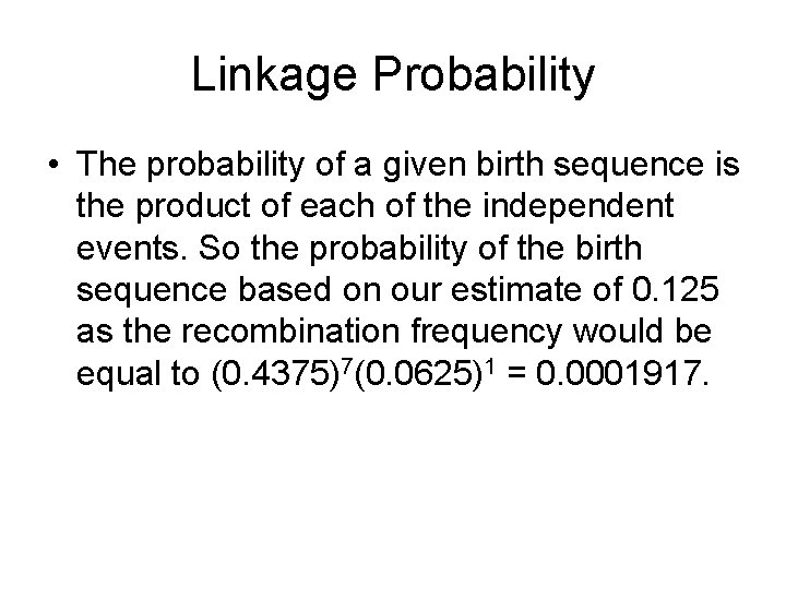
Linkage Probability • The probability of a given birth sequence is the product of each of the independent events. So the probability of the birth sequence based on our estimate of 0. 125 as the recombination frequency would be equal to (0. 4375)7(0. 0625)1 = 0. 0001917.

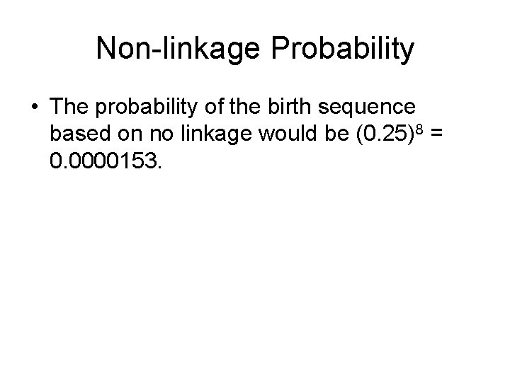
Non-linkage Probability • The probability of the birth sequence based on no linkage would be (0. 25)8 = 0. 0000153.

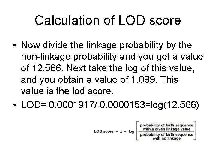
Calculation of LOD score • Now divide the linkage probability by the non-linkage probability and you get a value of 12. 566. Next take the log of this value, and you obtain a value of 1. 099. This value is the lod score. • LOD= 0. 0001917/ 0. 0000153=log(12. 566)

In practice, we would like to see a lod score greater that 3. 0. What this means is that the likelihood of linkage occurring at this distance is 1000 times greater that no linkage.

Case Control Studies Modified from Iris A. Granek, M. D. , M. S.

Case-control studies • Search for differences in allele frequency between disease carriers (cases) and non carriers (controls) with the assumption differences in frequencies are associated with disease outcome. • Can be applied to exposure to a chemical or a carcinogen instead of allele (genotypes).

Case Selection • Define the source population – residents of a geographic region – hospital inpatient or clinic • Strict case definition – inclusion criteria

Control Selection • Same source population as the cases • Choose the controls by random from the source population – spouses – associates – patients within the same facility – matched for certain criteria

Hospital Controls • Without regard to diagnosis • Excluding certain diseases • Including only diseases believed to be unrelated to the exposures (or alleles) being studied • Clinic patients from same hospital

Case Control Study Design Compares distribution of exposure cases (disease) vs. controls (without disease)

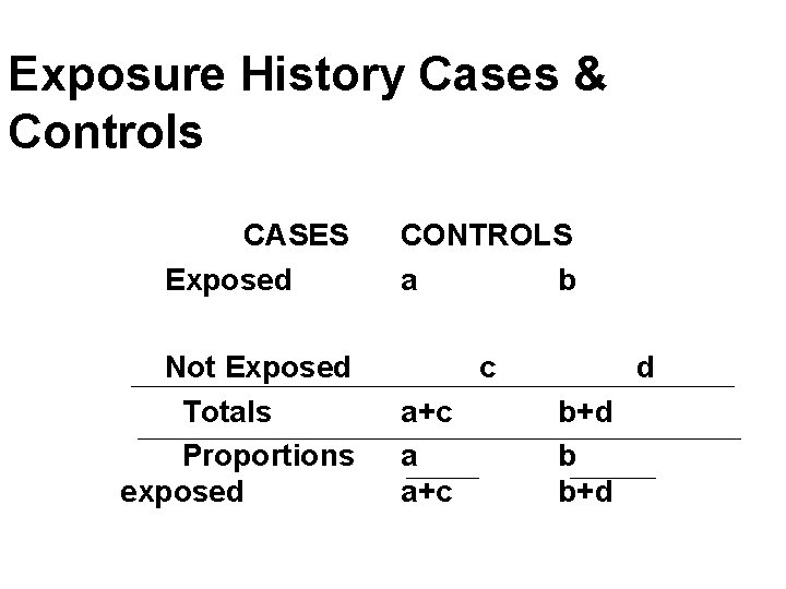
Exposure History Cases & Controls CASES Exposed Not Exposed Totals Proportions exposed CONTROLS a b c a+c a a+c d b+d b b+d

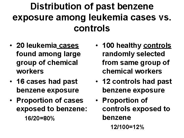
Distribution of past benzene exposure among leukemia cases vs. controls • 20 leukemia cases found among large group of chemical workers • 16 cases had past benzene exposure • Proportion of cases exposed to benzene: 16/20=80% • 100 healthy controls randomly selected from same group of chemical workers • 12 controls had past benzene exposure • Proportion of controls exposed to benzene 12/100=12%

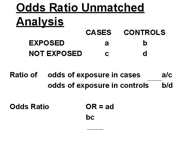
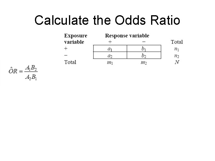
Odds Ratio Unmatched Analysis CASES EXPOSED a NOT EXPOSED c Ratio of CONTROLS b d odds of exposure in cases odds of exposure in controls Odds Ratio OR = ad bc a/c b/d

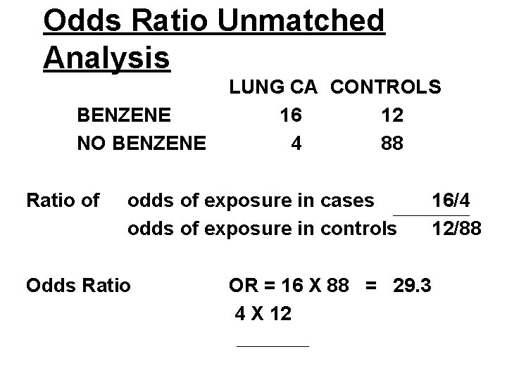
Odds Ratio Unmatched Analysis BENZENE NO BENZENE Ratio of LUNG CA CONTROLS 16 12 4 88 odds of exposure in cases odds of exposure in controls Odds Ratio OR = 16 X 88 = 29. 3 4 X 12 16/4 12/88

Odds Ratios • OR > 1 indicates a positive association between the factor and the disease – The lung cancer patients were 29 times more likely than the controls to have been exposed to benzene • OR < 1 indicates the factor is protective • OR = 1 indicates no association

95% Confidence Limits • 95% probability that the true value lies within the confidence interval or between the confidence limits • Odds ratios are statistically significant if they do not include 1 • OR = 7 (0. 5 - 15. 0) not statistically significant • OR = 7 (3. 0 - 12. 0) is statistically significant

Advantages of Case Control • Quick and Inexpensive • Optimal for rare diseases • Useful for diseases of long latency from exposure to disease development • Can evaluate multiple risk factors

Bias in Case Control Studies • Bias is a systematic error in the study that distorts the results & limits the validity of the conclusions. – Selection Bias – Confounding – Observation Bias (recall bias, interviewer bias, misclassification)

Selection Bias • Systematic errors arising from the way the subjects are selected – Study subjects are selected in a way that can misleadingly increase or decrease the magnitude of an association • Exposure of cases differs from exposure of all cases in source population or exposure of controls selected differs from non diseased in source population

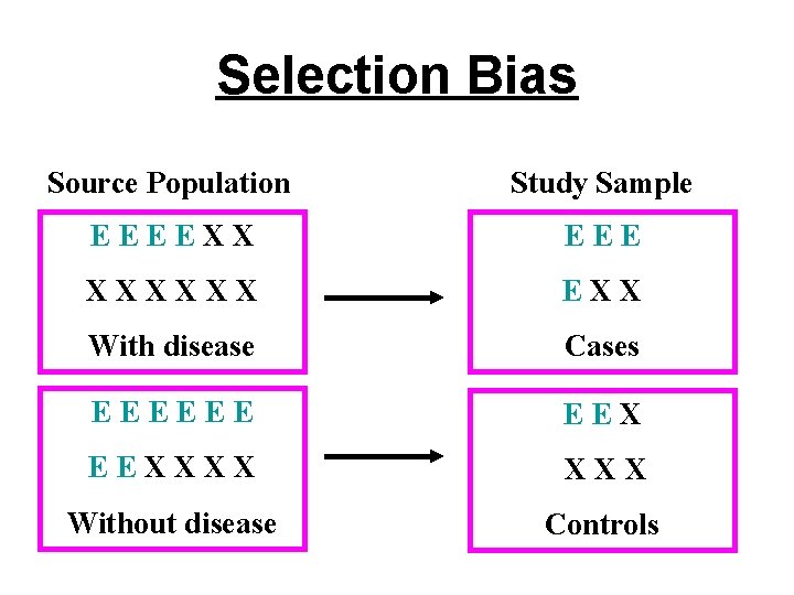
Selection Bias Source Population Study Sample EEEEXX EEE XXXXXX EXX With disease Cases EEEEEE EEXXXX Without disease Controls

Confounding • Distortion of the true relationship between the exposure and outcome due to a mutual relationship with another factor • Can be the reason for an apparent association & also may cause a true association to not be observed • Confounder must be associated with the outcome and the exposure

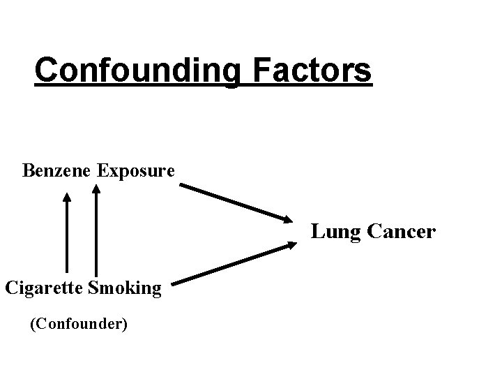
Confounding Factors Benzene Exposure Lung Cancer Cigarette Smoking (Confounder)

Controlling for Confounding The effect of confounding variables • can be controlled during the data analysis by various methods – stratification – multivariate analysis • can be controlled during the study design by matching controls and cases for the factor

Matched Case Control Design • Controls selected matched to cases on factors associated with the disease – age, sex, race, socioeconomic status • Makes the two groups similar on factors other than the exposure of interest • Cannot compare groups on matched factors • Must used matched analysis

Observation Bias • Interviewer (data collection) bias – keep data collection same for cases and controls • Misclassification Bias – incorrect characterization of exposure • Recall Bias – recall of exposures may be influenced by current disease status

Calculate the Odds Ratio

Esophagial cancer and alcohol

Fisher’s Exact Test http: //www. matforsk. no/ola/fisher. htm