Molecular Dynamics Verlet integrating equations of motion Langevin

Molecular Dynamics • • Verlet - integrating equations of motion Langevin dynamics – simulating water Monte Carlo Brownian

Integrating equations of motion • Newton’s 2 nd law • coupled first-order ODEs (IVP) – many-body problem; simulation • Runge-Kutta (4 th-order) cooling of a sphere: – 4 th-order: error decays with step size as O(h 5)

Verlet Algorithm • write forward and backward Taylor expansions to 3 rd-order: • calculate a from forces (deriv. of poten. energy): • estimate velocities from positions: • conservation of energy: • error is O(Dt 2) • nice property: symplectic integrator – conserves time-evolution of (perturbed) Hamiltonian – conserves volume in phase space

Leapfrog, Velocity Verlet • Velocity Verlet: calculate v from a (mid-step): • try to reduce errors to O(Dt 4) • Leapfrog

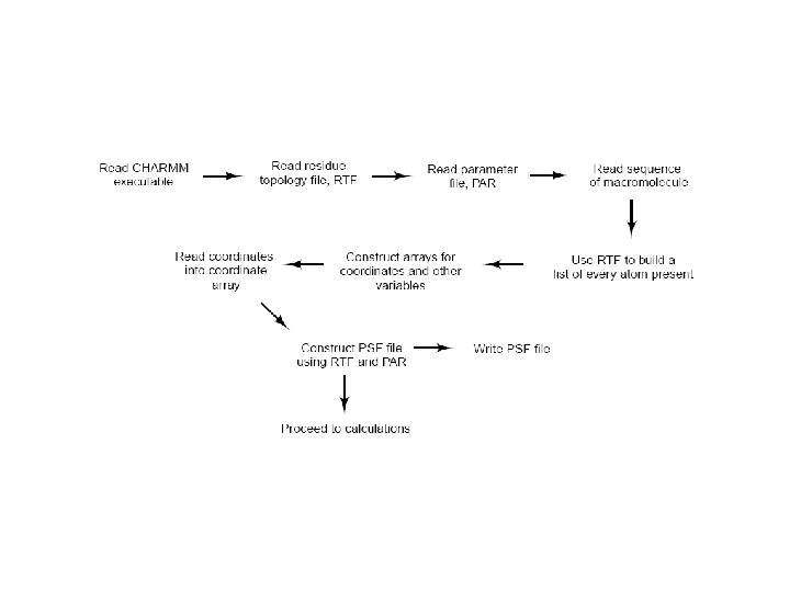
CHARMM • procedure – – – – build (H’s), solvate? minimize heat equilibrate production run, 100 ns / ~1 fs = 100, 000 iterations (quenching) analyze trajectory • minima (MC) • events and energy changes • time-correlations, spectra • Monte Carlo simulations – statistical mechanics, thermodynamic averages – kinetic energy

Loop flexing in triose phosphate isomerase • Derreumaux and Schlick (1998) • changes in energy correlated with 2 H-bonds. . . • importance of solvation (waters) – 1200 K LD in vac. , 1 opening event, 25 kcal/mol; interactions with water reduces the energy barrier

Unfolding of ß 2 microglobulin • Ma and Nussinov (2003) • amyloid formation • determine which sub-structures (betastrands) dissociate first • compare stability of N-terminal truncation and proteolytic cleavage native, 400 K native, 500 K trunc, 400 K

CHARMM resources • tutorials – http: //www. ch. embnet. org/MD_tutorial/ – http: //www. esi. umontreal. ca/accelrys/life/insight 2000. 1/ charmm_principles/Ch 04_mol_dyn. FM 5. html – http: //www. mdy. univie. ac. at/lehre/charmm/course 1/cour se 1 -1. html – http: //www. charmmtutorial. org/index. php/CHARMM: The _Basics • documentation (current version c 35 b 1) – http: //www. charmm. org/html/documentation/c 34 b 1/index. html • 180 -page online book by Robert Schleif – http: //gene. bio. jhu. edu/book. pdf

Scripts • • • charmm < minimize. inp > minimize. out PAR/TOP param files; PSF files (PDBs have coords, not connectivity) read write files: units (fortran) read the log files! (fix any errors) selection syntax copy coor comp trajectory files grep for “DYNA>”; monitor energy, temp in log file output time-correlation statistics (CORRel) – dihedrals, rms, energy. . .

Non-bonded cutoffs • ignore VDW, ES interactions beyond ~10Å – most forces are small at that range – greatly reduces run-time – may causes artifacts (non-smooth); may leak energy NBOND VSWITCH. . . CUTNb 16. 0 CTOFnb 12. CDIE EPS 1. CTONnb 8. • Particle-Mesh Ewald summation (PME) – allows calculation of total electrostatic energy (including long-range interactions) assuming periodic boundary conditions – model as lattice of protein-water boxes (like crystal) – use Fast Fourier-transform (in reciprocal space) to calculate product of potential at different points in unit cell with partial charges at all other points

Simulating Water Environment • implicit: distance-dependent dielectric (rdie=1) – extra 1/r in E: – dampens strength • Langevin dynamics – simulate friction of water via dissipative + random forces on surface atoms – g/m=t collision frequency, relaxation time – fluctuation-dispersion theorem: – in the limit of g=0, get Brownian dynamics

Explicit waters • explicit waters – each water adds 6 -9 degrees of freedom – water molecules strike side-chains on surface, impart random forces, exchange energy – dipoles interaction with surface atoms (H-bond) – add counter-ions to neutralize system • water box – periodic boundary conditions – pressure/volume changes

Water Molecules • Solvation – polarity (H-bonds) – density? velocity? residence times • Important for surface side-chains to not be in vacuum; helps them flex properly and reduce self-interactions • SPC model – 3 -points, H’s rigid (no bond stretch or bend) – 6 -dof rather than 9 – VDW interaction site centered on O • TIP 3 P model (Jorgensen et al. , 1983) – partial charges: q(O)=-0. 83, q(H)=+0. 415 • TIP 4 P – separate center of O charge from VDW center

diffusion, delectric permittivity, vibration spectra. . . TIP 4 P (Caleman) ice SPC/E

• quenching: lower temp or minimize at end of trajectory • SHAKE: constrain bonds to H’s, decreases dof • temperature drift (losses due to NB approx. ) – temperature scaling (artificial) – couple to heat bath – Nose-Hoover (Evans and Holian, 1985) • re-write equations of motion so T is a constant rather than E (scale momenta and time)

Thermodynamic ensembles • must generate proper ensemble for calculating thermodynamic averages (Monte Carlo) – standard simulations conserve energy (NVE), not temp – but proper (canonical) ensembles (NVT) have constant temp and variable energy; must couple to a heat bath • NVT: canonical ensemble – constant temperature, Helmholz free energy • NVE: micro-canonical ensemble – constant energy (microstate) – omega is count of microstates (related to entropy) • NPT (cpt) simulations – constant pressure (isobaric) – allow size of box to expand/contract (additional parameter) – Gibb’s free energy, E=U-TS+PV