MODULE II DEMAND ANALYSIS Susan Abraham Assistant Professor

MODULE II DEMAND ANALYSIS Susan Abraham Assistant Professor Dept of Economics Christian College

Demand � Demand is the desire for a commodity backed by ability and willingness to pay. � It requires: � A desire for the commodity must exist � The ability to pay for the commodity � The willingness to pay money.

Law of Demand � Ceteris paribus (other things remaining the same), the quantity of a good or service demanded varies inversely with it price. › inverse relationship between price and quantity demanded › movement is along the same demand curve. › other things which are assumed to be constant are the tastes or preferences of the consumer, the income of the consumer, the prices of related goods, etc. � If these other factors which determine demand also undergo a change, then the inverse price-demand relationship may not hold good

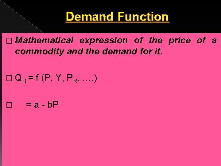
Demand Function � Mathematical expression of the price of a commodity and the demand for it. � QD = f (P, Y, PR, …. ) � = a - b. P

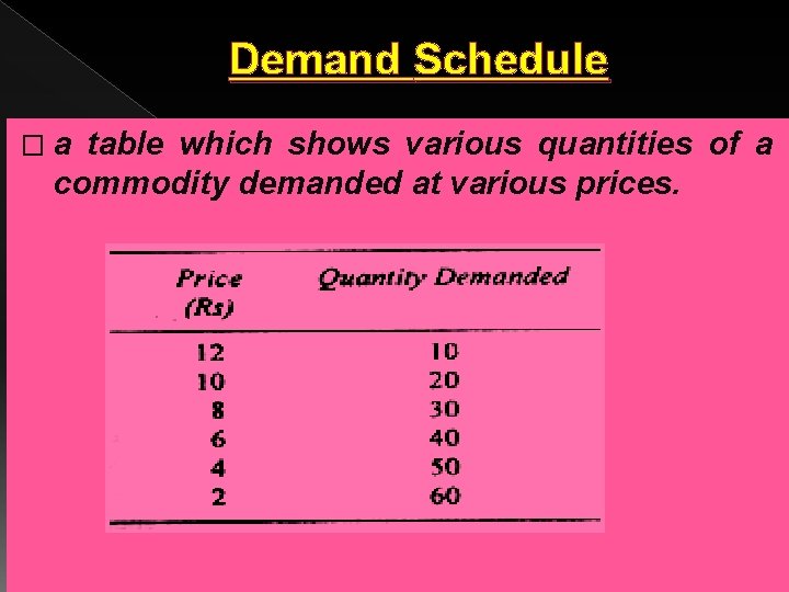
Demand Schedule � a table which shows various quantities of a commodity demanded at various prices.

Demand Schedule � A demand schedule can be of 2 types: › Individual demand schedule �shows the various quantities of a commodity demanded by a particular individual at different prices. › Market demand schedule (Industry demand Schedule) �shows the total quantity of a commodity demanded at different prices by all the buyers of the commodity in the market.

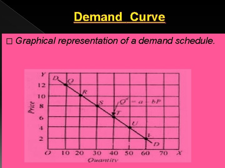
Demand Curve � Graphical representation of a demand schedule.

Demand Curve � Demand curve has a negative slope showing negative or inverse relationship between price and quantity demanded. � It may be a straight line (linear) or a curve (non linear) � Demand curves generally slopes downwards to the right.

Demand Function � A mathematical expression of the price of a commodity and the quantity demand for it. Demand Schedule � A table which shows various quantities of a commodity demanded at various prices. Demand Curve � A graphical representation schedule. of a demand

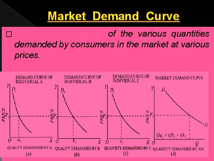
Market Demand Curve � Horizontal summation of the various quantities demanded by consumers in the market at various prices.

Reason for Downward Sloping Demand Curve 1. Diminishing Marginal Utility › A consumer pays for a commodity because it has utility. › He will buy it so long as his marginal utility from its consumption equals its price. PX = MUX › Suppose its price falls , then he needs to purchase more for his marginal utility to equal its price.

Reason for Downward Sloping Demand Curve 2. The Price Effect › Price effect comprises of : a) Income effect �When price increases, purchasing power of consumer falls, causing him to buy less. �Psychologically, the consumer feels richer. b) Substitution effect �When price increases, commodity becomes costlier in comparison with other substitute commodities, causing him to buy less. �Pyschologically the consumer feels poorer, hence he switches to a substitute and so buys less of the original good.

Reason for Downward Sloping Demand Curve 3. New Consumers › It is possible that at particular prices, some consumer may not be able to afford a commodity. › When price falls, they purchase more. 4. Different Uses › A commodity can be put to several uses. › Some are more important and some are less important. › When price of a commodity rises, they cut the less important uses and so purchase less. › E. g. Ponni Rice for idalis.

Exceptions to the Law of Demand 1. Veblen Goods (Goods having Prestige Value) � Some consumers measure the utility of a commodity entirely by its price › i. e. , for them, the greater the price of a commodity, the greater its utility. Such goods are called Veblen Goods. › E. g. diamonds, Rado / Tissot watches, Rolls Royce

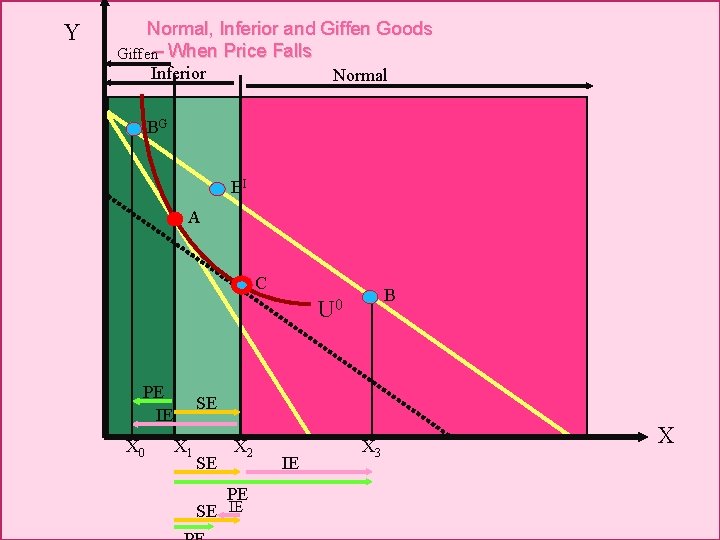
Exceptions to the Law of Demand 2. Giffen Goods: � A Giffen good is an inferior good with the unique characteristic that a fall in price decreases the quantity of the good demanded. › When the price of a Giffen good falls, instead of buying more of it, the consumer uses the increase in real income to purchase more of another good. � The demand curve will slope upward to the right and not downward. � This concept was the contribution of Sir Robert Giffen. � Cheap, necessary foods are examples of Giffens goods.

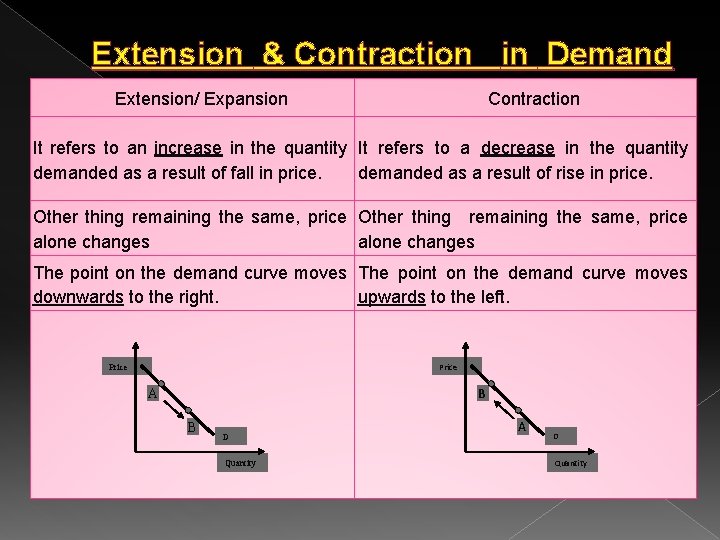
Extension & Contraction in Demand Extension/ Expansion Contraction It refers to an increase in the quantity It refers to a decrease in the quantity demanded as a result of fall in price. demanded as a result of rise in price. Other thing remaining the same, price Other thing remaining the same, price alone changes The point on the demand curve moves downwards to the right. upwards to the left. Price B A B D Quantity A D Quantity

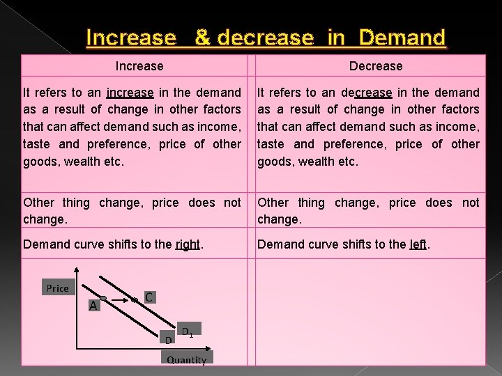
Increase & decrease in Demand Increase Decrease It refers to an increase in the demand as a result of change in other factors that can affect demand such as income, taste and preference, price of other goods, wealth etc. It refers to an decrease in the demand as a result of change in other factors that can affect demand such as income, taste and preference, price of other goods, wealth etc. Other thing change, price does not change. Demand curve shifts to the right. Price A C D D 1 Quantity Demand curve shifts to the left.

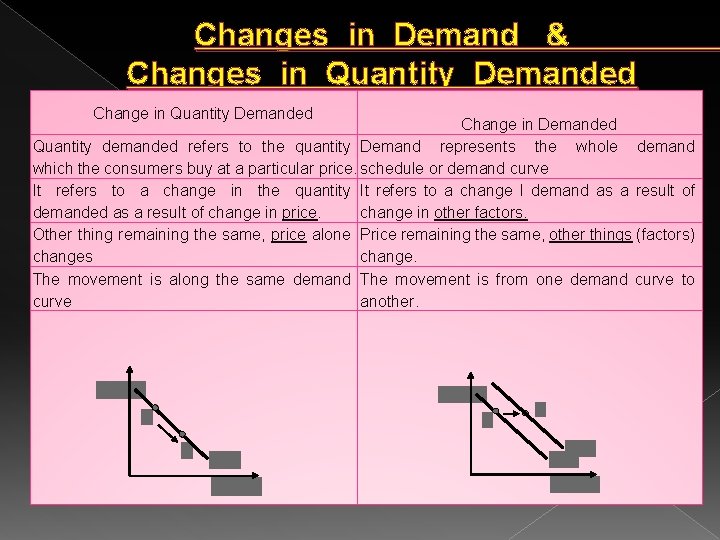
Changes in Demand & Changes in Quantity Demanded Change in Demanded Quantity demanded refers to the quantity Demand represents the whole demand which the consumers buy at a particular price. schedule or demand curve It refers to a change in the quantity It refers to a change I demand as a result of demanded as a result of change in price. change in other factors. Other thing remaining the same, price alone Price remaining the same, other things (factors) changes change. The movement is along the same demand The movement is from one demand curve to curve another.

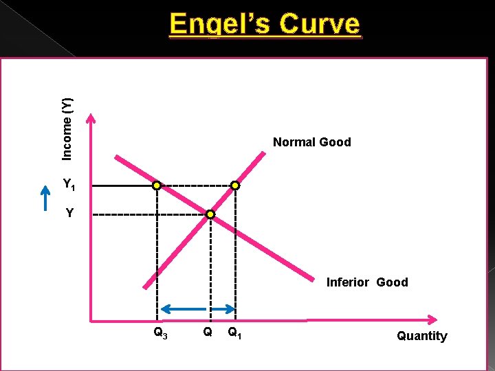
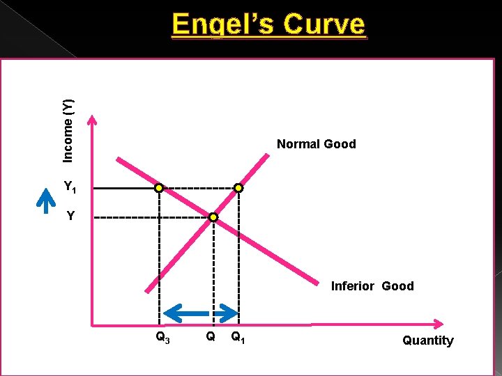
Determinants of Demand 1. Change in Income �Generally, when income increases there is increase in demand. Ø Normal Goods (Y ↑ → Qd↑ - Positive relation) �Sometimes, when income increases there is a decrease in demand. Ø Inferior Goods (Y ↑ → Qd↓ - Negative relation)

Determinants of Demand 2. Change in Price of Substitutes � When the price of a substitute good increases, the quantity demanded of that substitute good decreases. � People switch to other goods and the demand for those goods increases, even if its price remains the same. � Thus, when price of a substitute good increases, the quantity demanded of own good also increases. � (Ps ↑ → Qd↑- positive relation)

Determinants of Demand 3. Change in Price of Compliments � When the price of a complimentary good increases, the quantity demanded of that complimentary good decreases. � The demand for those goods which are used along with the complementary good also decreases, even if its price remains the same. � Thus, when price of a complimentary good increases, the quantity demanded of own good decreases. › � E. g. when price of mobiles increase there is decrease in the demand for sim cards (PC ↑ → Qd↑- negative relation)

Determinants of Demand 4. Change in Taste, Preferences and Habits �The demand for a commodity may change due to change in taste, fashion, preferences, etc. of the people in favour of that commodity. � 5. Change in Population � When population increases there is increase in new demand. � If there is decrease in population there is decrease in demand. � (Population ↑ → Qd↑ - Positive relation)

Elasticity of demand �Elasticity of demand, refers to the degree of responsiveness of quantity demanded of a goods to a change in its price, income and prices of related goods. �Alfred Marshall introduced the concept of elasticity in economic theory.

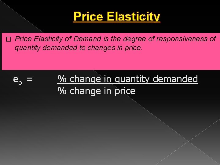
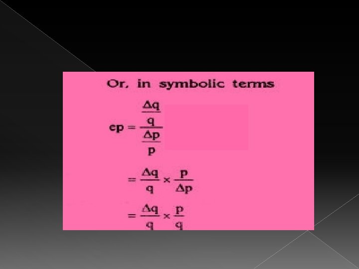
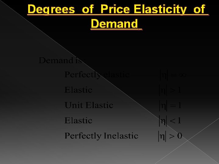
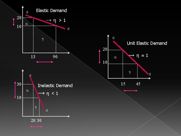
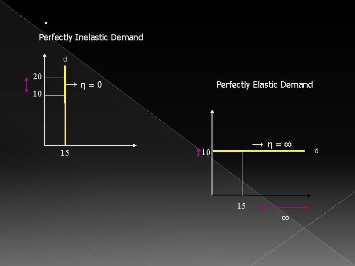
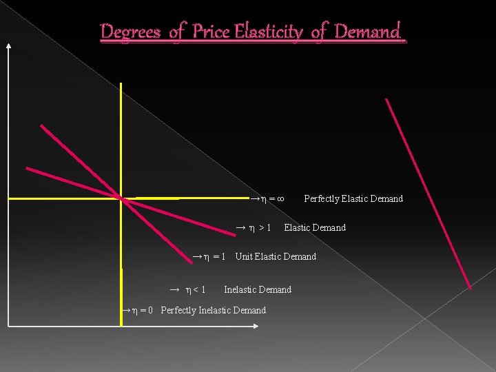
Price Elasticity � Price Elasticity of Demand is the degree of responsiveness of quantity demanded to changes in price. ep = % change in quantity demanded % change in price

Degrees of Price Elasticity of Demand

Elastic Demand d 20 10 → η >1 d d Unit Elastic Demand 20 13 → 90 η = 1 10 d 30 Inelastic Demand → η < 1 10 28 30 d 15 d 45

. Perfectly Inelastic Demand d 20 10 → η = 0 15 Perfectly Elastic Demand → 10 η = ∞ 15 ∞ d

Degrees of Price Elasticity of Demand → η = ∞ → η > 1 → η = 1 → η < 1 Perfectly Elastic Demand Unit Elastic Demand Inelastic Demand → η = 0 Perfectly Inelastic Demand

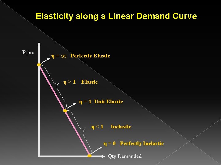
Elasticity along a Linear Demand Curve Price η = ∞ Perfectly Elastic η>1 Elastic η = 1 Unit Elastic η<1 Inelastic η = 0 Perfectly Inelastic Qty Demanded

Factors Affecting Price Elasticity 1. Nature of Commodity: �Necessity �comfort �luxury. � When a commodity is a necessity like food grains, vegetables, medicines, etc. , its demand is generally inelastic as it is required for human survival and its demand does not fluctuate much with change in price. � When a commodity is a comfort like fan, refrigerator, etc. , its demand is generally elastic as consumer can postpone its consumption. � When a commodity is a luxury like AC, DVD player, etc. , its demand is generally more elastic as compared to demand for comforts.

Factors Affecting Price Elasticity 2. Availability of Substitutes: a) perfect or close substitutes - Elastic b) Substitutes - More Elastic � E. g. a rise in the price of Pepsi encourages buyers to buy Coke and vice-versa. c) Few or no substitutes - Inelastic

Factors Affecting Price Elasticity 3. Income Level: 3. Higher income groups - inelastic �Lower income group - highly elastic 4. Level of Price: › Average prices of commodity high – Elastic demand › Average prices of commodity low– Inelastic demand �E. g. Needle, match box, etc. is inelastic demand.

Factors Affecting Price Elasticity 5. Share in Total Expenditure: • Greater the proportion of income spent on a commodity, greater the elasticity of demand for it and vice-versa. • Demand for necessities, goods like salt, needle, soap, match box, etc. tends to be inelastic as consumers spend a small proportion of their income on such goods. • If the proportion of income spent on a commodity is large, then demand for such a commodity will be elastic.

Factors Affecting Price Elasticity 6. Number of Uses: �If the commodity under consideration has several uses, then its demand will be inelastic. �When price of such a commodity increases, then it is generally put to only more urgent uses and, as a result, its demand falls. • E. g. electricity is a multiple-use commodity. Fall in its price will result in substantial increase in its demand, particularly in those uses (like AC, Heat convector, etc. ), where it was not employed formerly due to its high price.

Factors Affecting Price Elasticity 6. Postponement of Consumption: � Commodities like biscuits, soft drinks, etc. whose demand is not urgent, have highly elastic demand � Commodities with urgent demand like life saving drugs, have inelastic demand because of their immediate requirement.

Factors Affecting Price Elasticity 7. Time Period: › Price elasticity of demand is always related to a period of time. It can be a day, a week, a month, a year or a period of several years. �Demand is generally inelastic in the short period. �Demand is more elastic in long run

Factors Affecting Price Elasticity 8. Habits: › Commodities, which have become habitual necessities for the consumers, have less elastic (inelastic) demand. › Alcohol, tobacco, cigarettes, etc. 9. Recurring Demand: › Commodities characterized by recurring demand will be more elastic

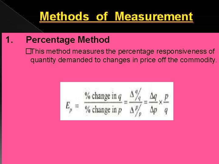
Methods of Measurement 1. Percentage Method �This method measures the percentage responsiveness of quantity demanded to changes in price off the commodity.

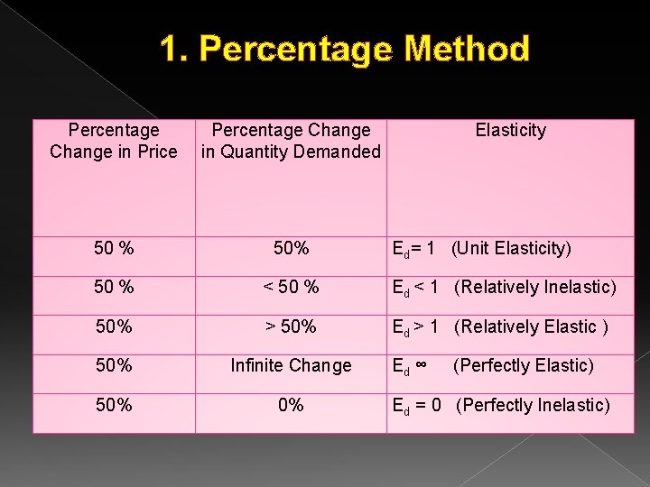
1. Percentage Method Percentage Change in Price Percentage Change in Quantity Demanded Elasticity 50 % < 50 % Ed < 1 (Relatively Inelastic) 50% > 50% Ed > 1 (Relatively Elastic ) 50% Infinite Change 50% 0% Ed= 1 (Unit Elasticity) Ed ∞ (Perfectly Elastic) Ed = 0 (Perfectly Inelastic)

2. The Point Method: � Elasticity is measured at a point on the demand curve.

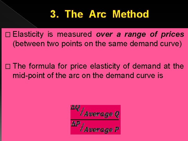
3. The Arc Method � Elasticity is measured over a range of prices (between two points on the same demand curve) � The formula for price elasticity of demand at the mid-point of the arc on the demand curve is

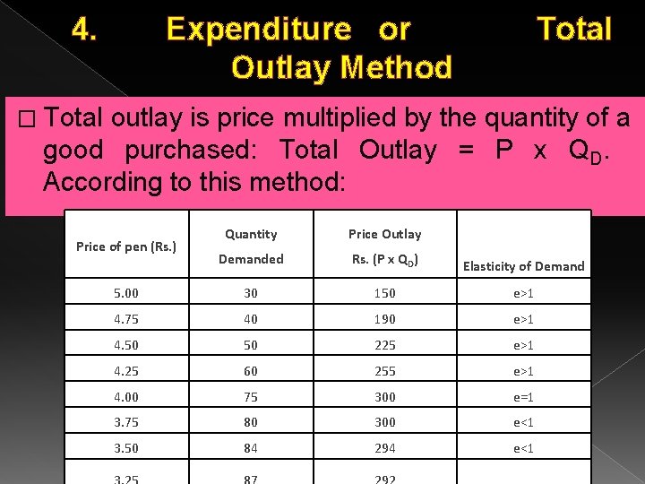
4. Expenditure or Total Outlay Method � Total outlay is price multiplied by the quantity of a good purchased: Total Outlay = P x QD. According to this method: Quantity Price Outlay Demanded Rs. (P x QD) Elasticity of Demand 5. 00 30 150 e>1 4. 75 40 190 e>1 4. 50 50 225 e>1 4. 25 60 255 e>1 4. 00 75 300 e=1 3. 75 80 300 e<1 3. 50 84 294 e<1 Price of pen (Rs. )

Uses of the Concept of Elasticity of Demand 1. 2. 3. 4. 5. In the determination of monopoly price: In the determination of prices of public utilities: In the determination of prices of joint products: In the determination of wages: In the determination of Government Policies a) While Granting Protection to industries b) While Deciding about Public Utilities c) d) 6. In Fixing Minimum Prices for Farm Products Importance to the Finance Minister: Importance in the Problems of International Trade

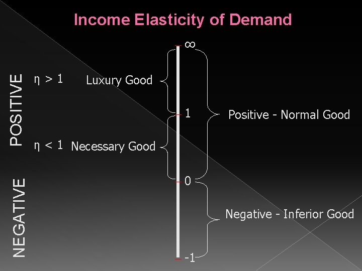
Income Elasticity of Demand � Income elasticity of demand measures the degree of responsiveness of quantity demanded of a good to changes in the consumer’s income. � ηi = % change in quantity demanded % change in income

Income Elasticity of Demand NEGATIVE POSITIVE ∞ η>1 Luxury Good 1 Positive - Normal Good η < 1 Necessary Good 0 Negative - Inferior Good -1

Income Elasticity of Demand � If income elasticity is positive (ηi >1) the good is a normal good (because a change in income and a change in demand move in the same direction). › If income elasticity is positive but less than 1 (ηi <1) the good is a necessary good. › If income elasticity is positive but greater than 1 (ηi >1) the good is a luxury good � If income elasticity is negative (ηi <0), (the good is an inferior good because a change in income and a change in demand move in opposite directions).

Cross Elasticity of Demand 1 Positive – Substitute Good + η>1 0 Negative – Complimentary Good -1 η<1

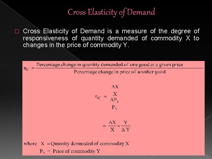
Cross Elasticity of Demand � Cross Elasticity of Demand is a measure of the degree of responsiveness of quantity demanded of commodity X to changes in the price of commodity Y.

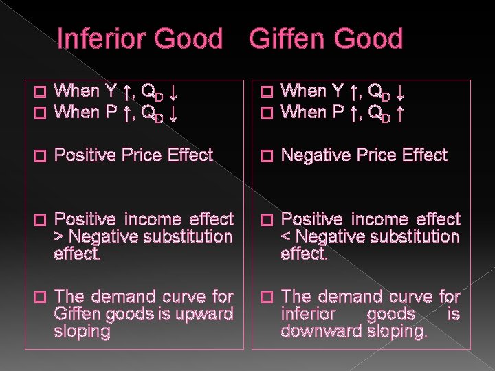
Inferior Good Giffen Good � � When Y ↑, QD ↓ When P ↑, QD ↓ � � When Y ↑, QD ↓ When P ↑, QD ↑ � Positive Price Effect � Negative Price Effect � Positive income effect > Negative substitution effect. � Positive income effect < Negative substitution effect. � The demand curve for Giffen goods is upward sloping � The demand curve for inferior goods is downward sloping.

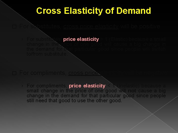
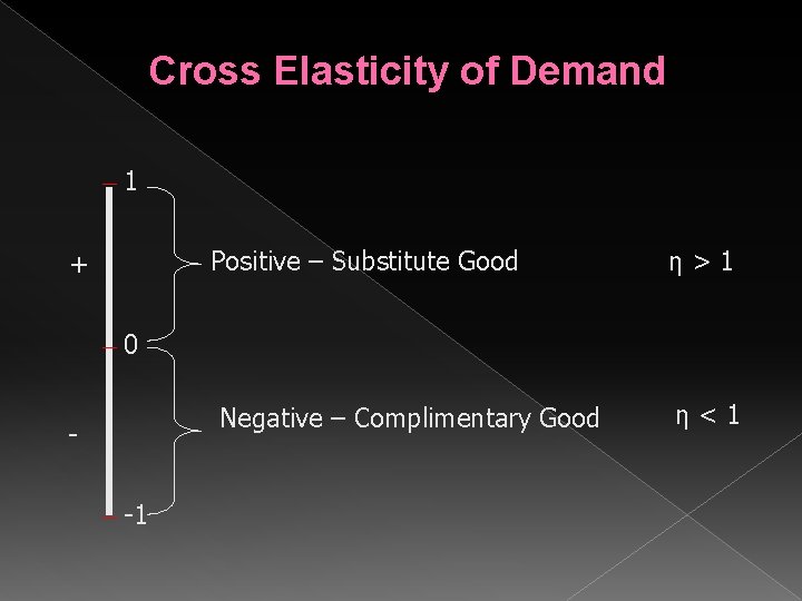
Cross Elasticity of Demand � For substitutes, cross price elasticity will be positive › For substitutes, price elasticity > 1 (Elastic) because a small change in the price of one good will cause a big change in the demand for that particular good since people will switch to/from substitute. � For compliments, cross price elasticity will be negative › For compliments, price elasticity < 1 (Inelastic) because a small change in the price of one good will not cause a big change in the demand for that particular good since people still need that good to use the other good.

Supply

Supply Function � A mathematical expression of the price of a commodity and the quantity supplied. Supply Schedule � A table which shows various quantities of a commodity supplied at various prices. Supply Curve � A graphical representation of a supply schedule.

Law of Supply � Ceteris paribus (other things remaining the same), the quantity of a good or service supplied varies inversely with it price. › Direct relationship between price and quantity supplied › movement is along the same supply curve. › other things which are assumed to be constant are the cost of production, tax rates, Government policy, etc. � If these other factors which determine supplyalso undergo a change, then the inverse price-demand relationship may not hold good

MODULE III Theory of Consumer Behaviour

The Theory of Consumer Behaviour �Theory of consumer behaviour is based on the assumption that consumers attempt to allocate limited money income among available goods and services so as to maximize utility/satisfaction.

Utility � Utility refers to the want satisfying capacity of a commodity. Characteristics: � Utility is subjective/not measurable � Utility is variable � Utility is different from usefulness � No legal or moral connotations � Utility derived from the first unit of a commodity is always positive.

The Theory of Consumer Behaviour � There are different approaches to theory of consumer behaviour: 1. Cardinal Utility Approach of Alfred Marshall 2. Ordinal Utility Approach of Hicks and Allen 3. Ordinal Utility Approach of Paul Samuelson

Cardinal Utility Theory � School of Utilitarianism. � According to them, Utility can be measured and compared by assigning numbers. � The Utility function that tells exactly by how much a bundle is preferred over another is a Cardinal Utility function. Ordinal Utility Theory � Utility can not be measured precisely but it can be ranked in order of preference relative to one other. � Once preferences are stated, a rational consumer will always stick with that choice. � It is the ordinal utility function that gives rise to indifference curves.

Cardinal Utility Assumptions: � The Cardinal Measurability of Utility. � Constancy of the Marginal Utility of Money. � No change in income of the consumer. � Taste & fashion is constant. � No close substitutes

Cardinal Utility Analysis � The term utility was introduced by British philosopher Jeremy Bentham. � Utility is the want satisfying power of a commodity. � Classical and Neoclassical economists used the concept of Cardinal Utility. › According to them a consumer could assign a cardinal number to each commodity when consumed. › The unit of measurement of utility in terms of numbers is called which is an imaginary unit. util,

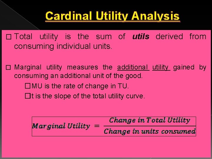
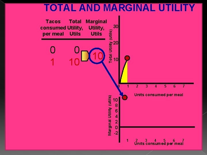
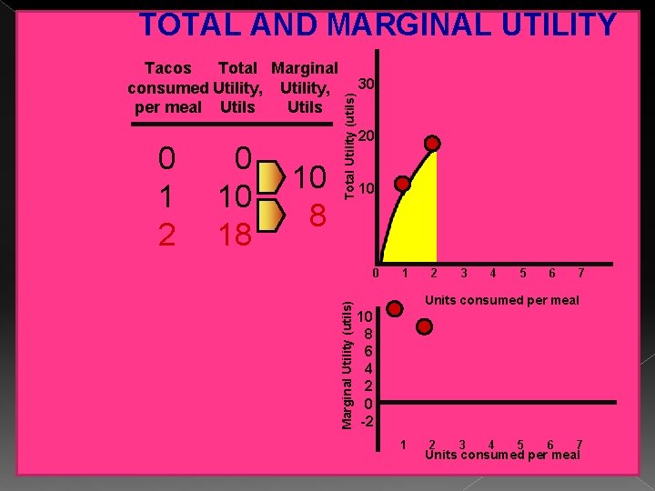
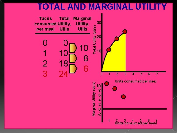
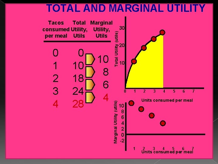
Cardinal Utility Analysis � Total utility is the sum of utils derived from consuming individual units. � Marginal utility measures the additional utility gained by consuming an additional unit of the good. � MU is the rate of change in TU. �It is the slope of the total utility curve.

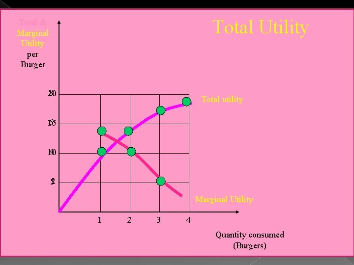
Total Utility Total & Marginal Utility per Burger 8 20 Total utility 6 15 4 10 2 5 Marginal Utility 1 2 3 4 Quantity consumed (Burgers)

� The founders of cardinal utility analysis have developed two laws which occupy an important place in economic theory and have several applications and uses. Law of Diminishing Marginal Utility 2. Law of Equi-Marginal Utility. 1. � It is with the help of these two laws about consumer’s behaviour that the exponents of cardinal utility analysis have derived the law of demand.

Law of Diminishing Marginal Utility Assumptions 1. Units of consumption are homogeneous (standardised). 2. Consumption is continuous. No breaks. 3. Taste and preference of the consumer remains constant. 4. Rationality: The consumer is rational. The objective of the consumer is to maximise his utility subject to his limited income. 5. Cardinal Utility: Utility from each commodity is cardinally measureable by the consumer (in utils). 6. Total Utility is Additive: The TU derived from a basket of commodities is the sum of the utilities derived from individual commodities. 7. Marginal Utility of Money is Constant: Utility of a commodity can be measured in terms of money. Marginal utility of money is assumed constant. (If the MU of money changes as income changes, then money cannot be used as a standard measure of utility. )

Law of Diminishing Marginal Utility � This law was put forward by Alfred Marshall. � According to him, the Law of Diminishing Marginal Utility states that ‘the additional benefit which a person derives from a given increase in his stock of a thing diminishes with every increase in the stock that he already has’.

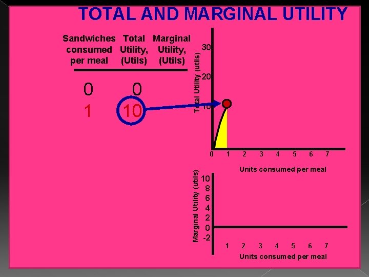
TOTAL AND MARGINAL UTILITY 0 10 Total Utility (utils) 0 1 30 20 10 0 1 2 3 4 5 6 7 Marginal Utility (utils) Sandwiches Total Marginal consumed Utility, per meal (Utils) Units consumed per meal 10 8 6 4 2 0 -2 1 2 3 4 5 6 7 Units consumed per meal

TOTAL AND MARGINAL UTILITY 0 10 10 Total Utility (utils) 0 1 30 20 10 0 1 2 3 4 5 6 7 Marginal Utility (utils) Tacos Total Marginal consumed Utility, per meal Utils Units consumed per meal 10 8 6 4 2 0 -2 1 2 3 4 5 6 7 Units consumed per meal

TOTAL AND MARGINAL UTILITY 0 10 18 10 8 Total Utility (utils) 0 1 2 30 20 10 0 1 2 3 4 5 6 7 Marginal Utility (utils) Tacos Total Marginal consumed Utility, per meal Utils Units consumed per meal 10 8 6 4 2 0 -2 1 2 3 4 5 6 7 Units consumed per meal

TOTAL AND MARGINAL UTILITY 0 10 18 24 10 8 6 Total Utility (utils) 0 1 2 3 30 20 10 0 1 2 3 4 5 6 7 Marginal Utility (utils) Tacos Total Marginal consumed Utility, per meal Utils Units consumed per meal 10 8 6 4 2 0 -2 1 2 3 4 5 6 7 Units consumed per meal

TOTAL AND MARGINAL UTILITY 0 10 18 24 28 10 8 6 4 Total Utility (utils) 0 1 2 3 4 30 20 10 0 1 2 3 4 5 6 7 Marginal Utility (utils) Tacos Total Marginal consumed Utility, per meal Utils Units consumed per meal 10 8 6 4 2 0 -2 1 2 3 4 5 6 7 Units consumed per meal

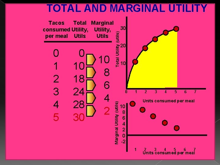
TOTAL AND MARGINAL UTILITY 0 10 18 24 28 30 10 8 6 4 2 Total Utility (utils) 0 1 2 3 4 5 30 20 10 0 1 2 3 4 5 6 7 Marginal Utility (utils) Tacos Total Marginal consumed Utility, per meal Utils Units consumed per meal 10 8 6 4 2 0 -2 1 2 3 4 5 6 7 Units consumed per meal

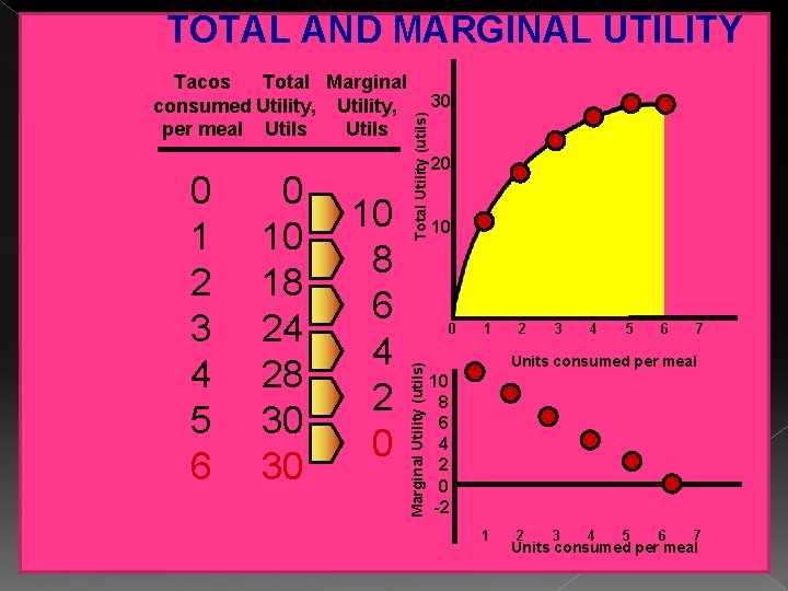
TOTAL AND MARGINAL UTILITY 0 10 18 24 28 30 30 10 8 6 4 2 0 Total Utility (utils) 0 1 2 3 4 5 6 30 20 10 0 1 2 3 4 5 6 7 Marginal Utility (utils) Tacos Total Marginal consumed Utility, per meal Utils Units consumed per meal 10 8 6 4 2 0 -2 1 2 3 4 5 6 7 Units consumed per meal

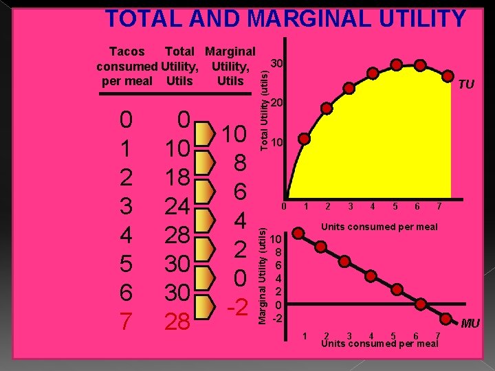
TOTAL AND MARGINAL UTILITY 0 10 18 24 28 30 30 28 10 8 6 4 2 0 -2 Total Utility (utils) 0 1 2 3 4 5 6 7 30 TU 20 10 0 1 2 3 4 5 6 7 Marginal Utility (utils) Tacos Total Marginal consumed Utility, per meal Utils Units consumed per meal 10 8 6 4 2 0 -2 MU 1 2 3 4 5 6 7 Units consumed per meal

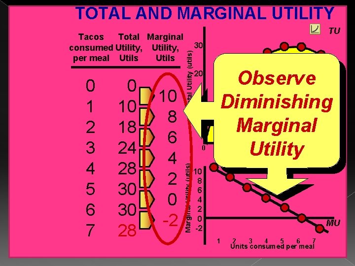
TOTAL AND MARGINAL UTILITY 0 10 18 24 28 30 30 28 10 8 6 4 2 0 -2 30 Total Utility (utils) 0 1 2 3 4 5 6 7 TU 20 10 Observe Diminishing Marginal Utility 0 1 2 3 4 5 6 7 Marginal Utility (utils) Tacos Total Marginal consumed Utility, per meal Utils Units consumed per meal 10 8 6 4 2 0 -2 MU 1 2 3 4 5 6 7 Units consumed per meal

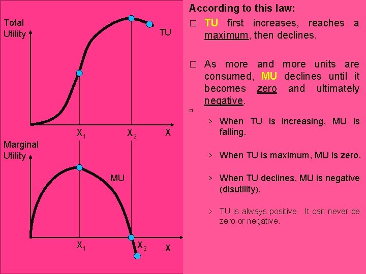
Total Utility TU According to this law: � TU first increases, reaches a maximum, then declines. � � Marginal Utility X 1 X 2 X As more and more units are consumed, MU declines until it becomes zero and ultimately negative. . › When TU is increasing, MU is falling. › When TU is maximum, MU is zero. › When TU declines, MU is negative (disutility). MU › TU is always positive. It can never be zero or negative. X 1 X 2 X

Law of Diminishing Marginal Utility � It is MU and not TU that determines the price of a commodity. � A consumer buys a commodity when Marginal Utility from the commodity is equal to its price (MU = P). �If MU > P, consumer will consume more and more units until MU = P. �If MU < P, consumer will consume less until MU = P. � MU declines because of the following reasons: 1. Commodities are imperfect substitutes for each other. 2. Although wants are unlimited, individual wants are satiable (satisfiable).

Limitations /Exceptions to the Law of Diminishing Marginal Utility 1. Other things should remain the same. 2. The law does not work in the case of addicts, misers, drunkards, etc. 3. It does not work in the case of Prestige Goods, Hobbies and Rare Things. 4. The law is not applicable to money.

The Law of Equi-Marginal Utility � This law was presented in 19 th century by an Australian economist, H. H. Gossen. Assumptions: 1. 2. 3. 4. 5. 6. 7. 8. The consumer is a rational being. Consumer has a given income. There are only two goods X and Y on which a consumer can spend the given income. Prices of the two goods are given (fixed). Marginal utility of the two commodities are independent of each other and diminishes with each additional unit consumed. Marginal utility of money remains constant for the consumer as he spends more and more of it on the purchase of goods X and Y. The two good are substitutes. Goods are divisible into small units.

Law of Equi-Marginal Utility � According to this Law, consumer behaviour will be governed by two factors: 1. Marginal utilities of the goods (MU) 2. Prices of two goods (P)

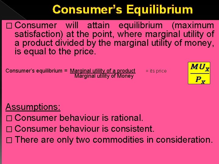
Consumer’s Equilibrium � Consumer will attain equilibrium (maximum satisfaction) at the point, where marginal utility of a product divided by the marginal utility of money, is equal to the price. Consumer’s equilibrium = Marginal utility of a product = its price Marginal utility of Money Assumptions: � Consumer behaviour is rational. � Consumer behaviour is consistent. � There are only two commodities in consideration.

Consumer’s Equilibrium � The consumer can either buy x or retain his money income Y. � The consumer is in equilibrium when the marginal utility of x is equated to its market price (Px). � Symbolically MUX = Px � If the marginal utility of x is greater than its price, the consumer can increase his welfare by purchasing more units of x. Similarly if the marginal utility of x is less than its price the consumer can increase his total satisfaction by cutting down the quantity of x and keeping more of his income unspent. � Therefore, he attains the maximization of his utility when MUX = Px. �

� If there are more commodities, the condition for the equilibrium of the consumer is the equality of the ratios of the marginal utilities of the individual commodities to their prices

Law of Equi-Marginal Utility � Marginal utility of money expenditure is equal to the marginal utility of the good divided by the price of the good.

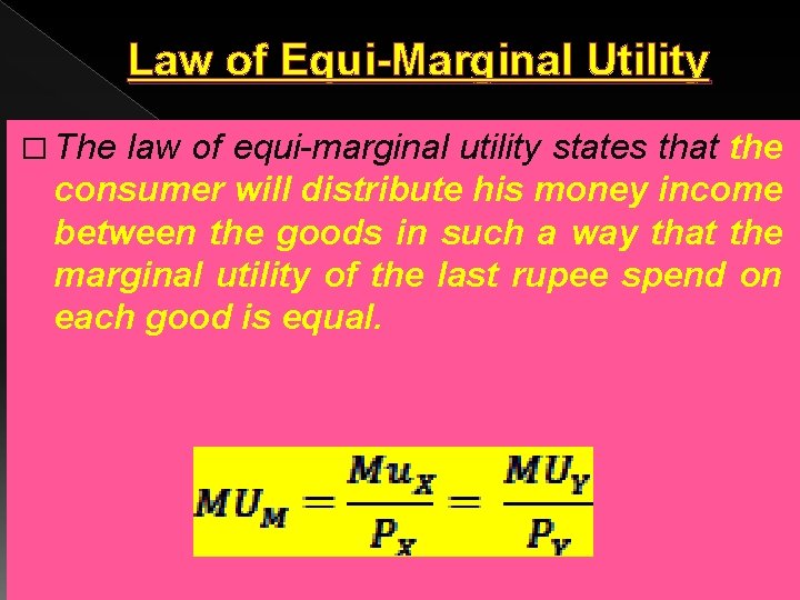
Law of Equi-Marginal Utility � The law of equi-marginal utility states that the consumer will distribute his money income between the goods in such a way that the marginal utility of the last rupee spend on each good is equal.

The Law of Equi-Marginal Utility � The consumer can get maximum utility by allocating income among commodities in such a way that the last rupee spent on each item provides the same marginal utility.

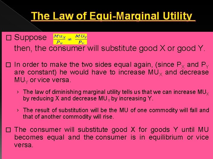
The Law of Equi-Marginal Utility � Suppose then, the consumer will substitute good X or good Y. � In order to make the two sides equal again, (since PX and PY are constant) he would have to increase MUX and decrease MUY or vice versa. › The law of diminishing marginal utility tells us that we can increase MUX by reducing X and decrease MUY by increasing Y. › The result of substitution will be the MU of one commodity will fall and that of another commodity will rise. � The consumer will substitute good X for goods Y until MU becomes equal and the consumer is in equilibrium or vice versa.

Derivation of Demand Curve � The consumer will be in equilibrium when marginal utility of money expenditure on each goods is the same. › As the units of the commodity consumed increases, MU declines. › Therefore, each additional unit of the good gives him lesser and lesser satisfaction. › This means that additional units will be purchased only if the price is reduced.

Limitations of Law of Equi-Marginal Utility � It is difficult for the consumer to know the marginal utilities from different commodities because utility cannot be measured. � Consumer are ignorant and therefore are not in a position to arrive at an equilibrium. � It does not apply to indivisible and inexpensive commodity.

Derivation of Demand Curve � In the cardinal utility theory, the demand curve is derived from the Marginal Utility Curve. � The Marginal Utility curve graphically shows the additional utility gained by consuming an additional unit of a good. � Diminishing marginal utility is one of the major causes of the downward slope of the demand curve. � The Neo-Classical economists uses this concept to explain how the demand curve of an individual is derived.

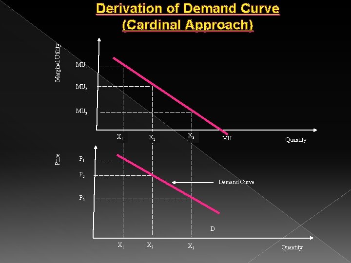
Marginal Utility Derivation of Demand Curve (Cardinal Approach) MU 1 MU 2 MU 3 Price X 1 X 2 X 3 MU Quantity P 1 P 2 Demand Curve P 3 D X 1 X 2 X 3 Quantity

Limitations/Criticism of Neo-classical Theory of Demand (Cardinal Utility Analysis) 1. Utility is not cardinally measurable. The satisfaction derived from various commodities cannot be measured in numbers. 2. MU of money is not constant. As income increases the MU of money changes. 3. Utilities are interdependent. The theory is based on the assumption that utilities of different commodities are independent. But in real life, utility of a commodity is dependent on other commodities like compliments and substitutes. 4. Failure to distinguish income effect and substitution effect. Price change has an income effect and a substitution effect. Cardinal theory does not consider this. 5. Failure to explain consumer behaviour in the case of Giffen goods. The positively sloping demand curve of a Giffen good is an exception of Marshall’s Law of Demand.

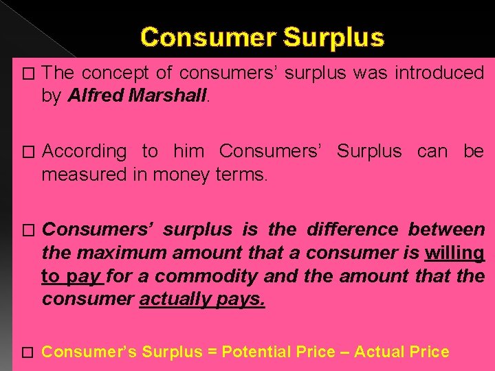
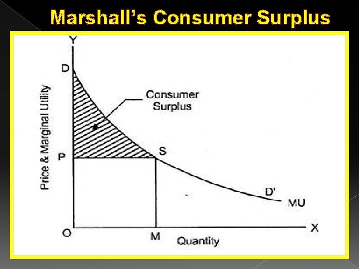
Consumer Surplus � The concept of consumers’ surplus was introduced by Alfred Marshall. � According to him Consumers’ Surplus can be measured in money terms. � Consumers’ surplus is the difference between the maximum amount that a consumer is willing to pay for a commodity and the amount that the consumer actually pays. � Consumer’s Surplus = Potential Price – Actual Price

Consumer Surplus � According to Marshall: Consumer Surplus is “the excess of the price which a person would be willing to pay rather than go without the thing over that which he actually does have to pay. ” � E. g. Suppose, a student goes to buy a book. � He is willing to pay Rs. 20 for the book. � But he gets the book for Rs. 15. � Thus, he has saved Rs. 5. This is called Consumer’s Surplus.

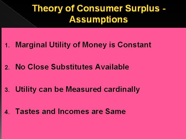
Theory of Consumer Surplus - Assumptions 1. Marginal Utility of Money is Constant 2. No Close Substitutes Available 3. Utility can be Measured cardinally 4. Tastes and Incomes are Same

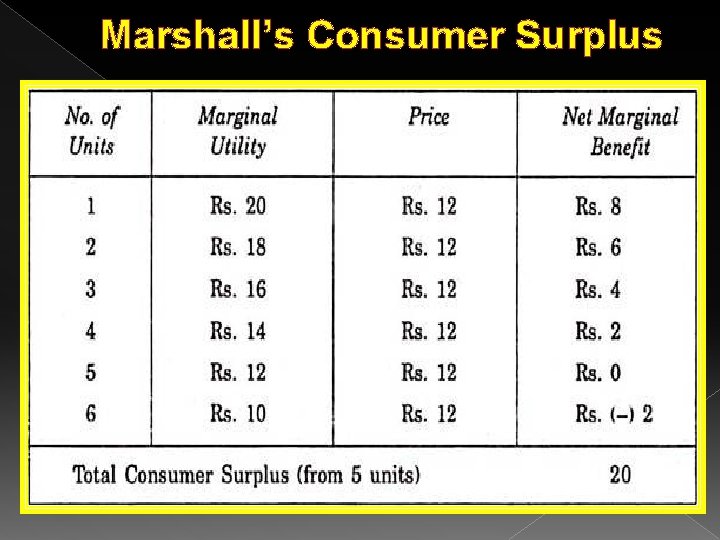
Marshall’s Consumer Surplus

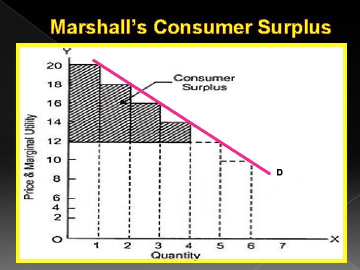
Marshall’s Consumer Surplus D

Marshall’s Consumer Surplus

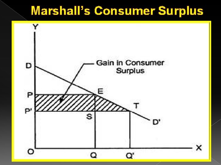
Marshall’s Consumer Surplus

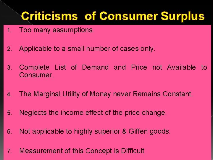
Criticisms of Consumer Surplus 1. Too many assumptions. 2. Applicable to a small number of cases only. 3. Complete List of Demand Price not Available to Consumer. 4. The Marginal Utility of Money never Remains Constant. 5. Neglects the income effect of the price change. 6. Not applicable to highly superior & Giffen goods. 7. Measurement of this Concept is Difficult

Economic Surplus � In economics, consumers and producers obtain “benefit surpluses” through market transactions. � Economic surplus, also known as Marshallian surplus, was named after Alfred Marshall

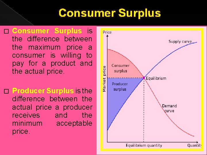
Consumer Surplus � Consumer Surplus is the difference between the maximum price a consumer is willing to pay for a product and the actual price. � Producer Surplus is the difference between the actual price a producer receives and the minimum acceptable price.

Indifference Curve Analysis

Ordinal Approach � There are two approaches explaining theory of consumer behaviour based on ordinal utility. � They are 1. Indifference Curve Approach 2. Revealed Preference Theory. � These approaches rejected the cardinal utility concept of the neo-classical school. � Ordinal utility means that the consumer is ranking or ordering the utilities of goods rather than measuring them in terms of cardinal numbers.

Indifference Curve Analysis � It was elaborated and popularised by two British economists, J. R. Hicks and R. G. D. Allen. � In indifference theory the consumer’s tastes or preferences are represented by indifference curves.

Assumptions of Ordinal Utility Theory 1. The consumer consumes only two goods (X and Y). The goods are homogenous and perfectly divisible. 2. Rationality: The consumer is rational. The objective of the consumer is to maximize his/her utility subject to (i) his limited income and (ii) the prices of the commodities. 3. Utility is Ordinal: The consumer can only rank his preferences 1 st, 2 nd, 3 rd and so on according to the satisfaction. He cannot cardinally measure them. 4. Diminishing Marginal Rate of Substitution: It means that the quantity of Y the consumer is willing to sacrifice for each additional unit of X becomes successively smaller. 5. Dependent Utilities: Total utility of the consumer depends on the quantities of the commodities consumed. 6. Consumers’ Preference is Transitive: If the consumer prefers bundle A to B and B is preferred to C, then he prefers A to C.

Indifference Curve � Indifference curve is a tool for analysing consumer behaviour. � An indifference curve shows various combinations of two goods that yield the same level of satisfaction (utility) to the consumer. � Each combination of goods on an indifference curve gives the consumer the same level of utility. � Since they give the same level of utility, the consumer is indifferent among all combinations of goods on an indifference curve. The slope of the IC is given by the Marginal Rate of Substitution.

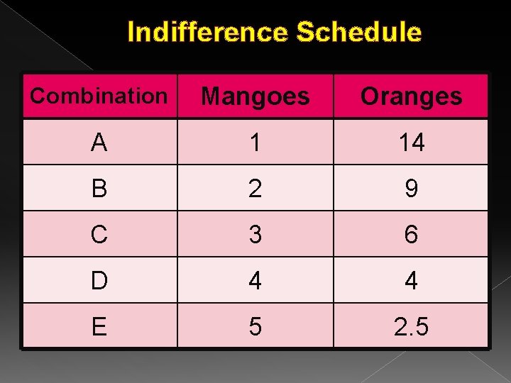
Indifference Schedule Combination Mangoes Oranges A 1 14 B 2 9 C 3 6 D 4 4 E 5 2. 5

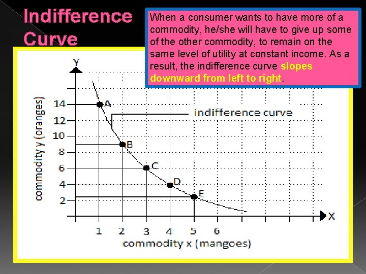
Indifference Curve When a consumer wants to have more of a commodity, he/she will have to give up some of the other commodity, to remain on the same level of utility at constant income. As a result, the indifference curve slopes downward from left to right.

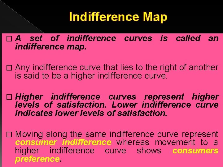
Indifference Map � A set of indifference curves is called an indifference map. � Any indifference curve that lies to the right of another is said to be a higher indifference curve. � Higher indifference curves represent higher levels of satisfaction. Lower indifference curve indicates lower levels of satisfaction. � Moving along the same indifference curve represent consumer indifference whereas movement to a higher indifference curve shows consumers preference.

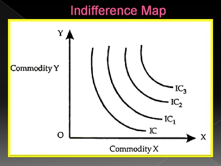
Indifference Map

Properties of Indifference Curve 1. All combinations of goods along the IC give the consumer the same level of satisfaction. › Since they give the same level of utility, the consumer is indifferent among all combinations of goods on an indifference curve.

Properties of Indifference Curve 2. Indifference Curves have a negatively slope: �The IC at any point represents the individual’s willingness to pay for X in terms of Y. �To consume additional units of X, the consumer has to sacrifice additional units of Y.

Properties of Indifference Curve 3. The slope of an indifference curve decreases as we move down the indifference curve. › The willingness of the consumer to sacrifice more and more units of one commodity diminishes as he goes on substituting one and gets more and more of the other. › The slope is steeper in the beginning and becomes flatter later on as the individual becomes more and more reluctant to sacrifice Y for additional units of X.

Properties of Indifference Curve 4. Indifference Curves are Convex to the origin: �Convexity of indifference is due to the Diminishing Marginal Rate of Substitution. �The degree of convexity of an indifference curve depends on whether the two goods are compliment, substitutes or unrelated to each other.

Properties of Indifference Curve 5. Indifference Curves cannot intersect or be Tangent: �Indifference curve cannot intersect. �They are always parallel to each other. �By definition, point A on one indifference curve cannot give the same utility as both B and C on another indifference curve. This would be a logical impossibility.

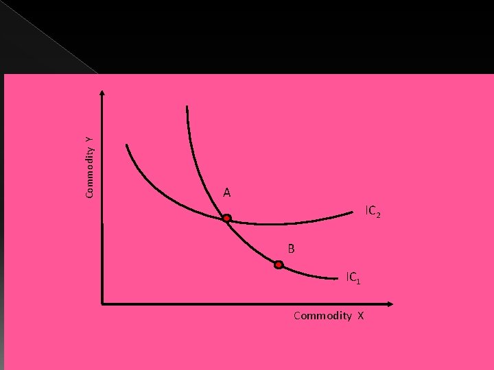
Commodity Y . A IC 2 B IC 1 Commodity X

Properties of Indifference Curve 6. Higher Indifference Curves represent Higher Levels of satisfaction. � An indifference curve that lies farther from the origin (higher IC) represents a greater level of satisfaction.

Properties of Indifference Curve 7. Indifference Curves are Everywhere: › Density of indifference curves means that there an infinite number of indifference curves between any two indifference curves.

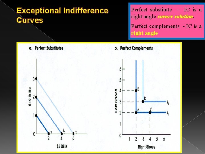
Exceptional Indifference Curves Perfect substitute - IC is a right angle corner solution. Perfect complements - IC is a right angle

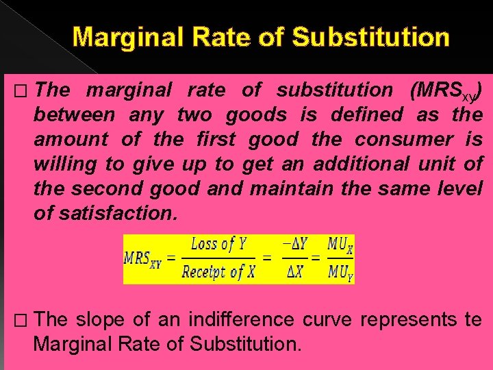
Marginal Rate of Substitution � The marginal rate of substitution (MRSxy) between any two goods is defined as the amount of the first good the consumer is willing to give up to get an additional unit of the second good and maintain the same level of satisfaction. � The slope of an indifference curve represents te Marginal Rate of Substitution.

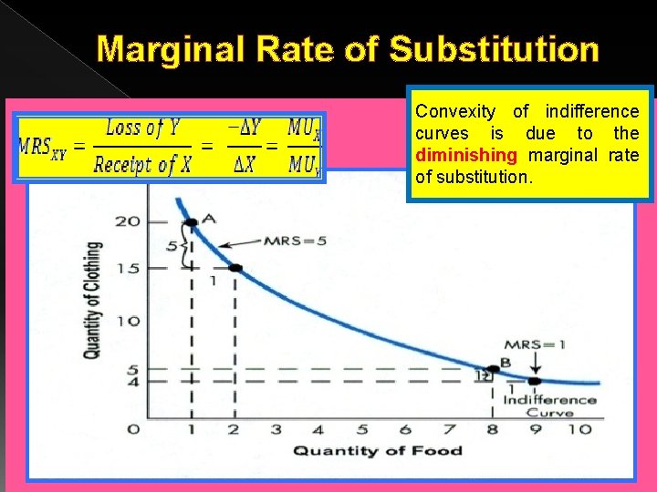
Marginal Rate of Substitution Convexity of indifference curves is due to the diminishing marginal rate of substitution.

Budget Line / Price Line (Budget Constraint) � A consumer’s income decides what combination of commodities he can buy. � Budget line is a curve connecting all combinations of two goods that a consumer can purchase with a given income or budget constraint.

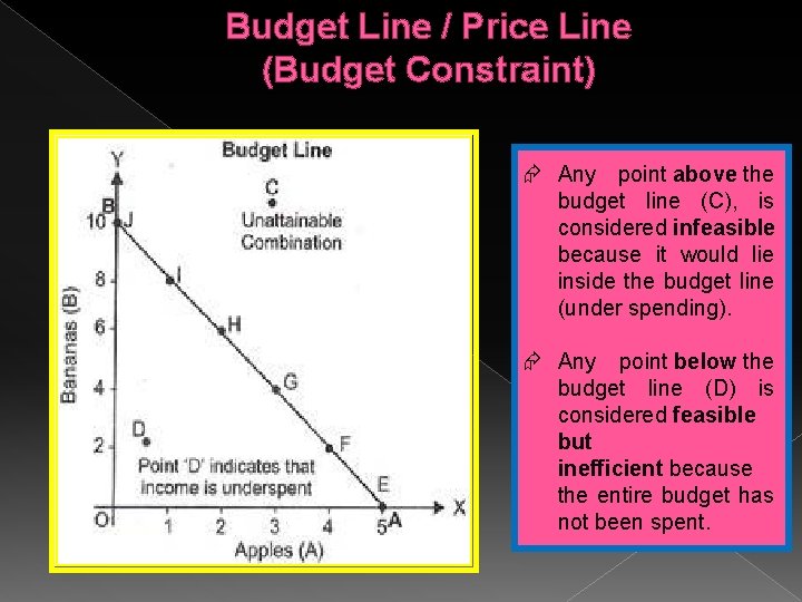
Budget Line / Price Line (Budget Constraint) Any point above the budget line (C), is considered infeasible because it would lie inside the budget line (under spending). Any point below the budget line (D) is considered feasible but inefficient because the entire budget has not been spent.

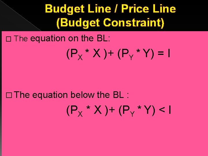
Budget Line / Price Line (Budget Constraint) � The equation on the BL: (PX * X )+ (PY * Y) = I � The equation below the BL : (PX * X )+ (PY * Y) < I

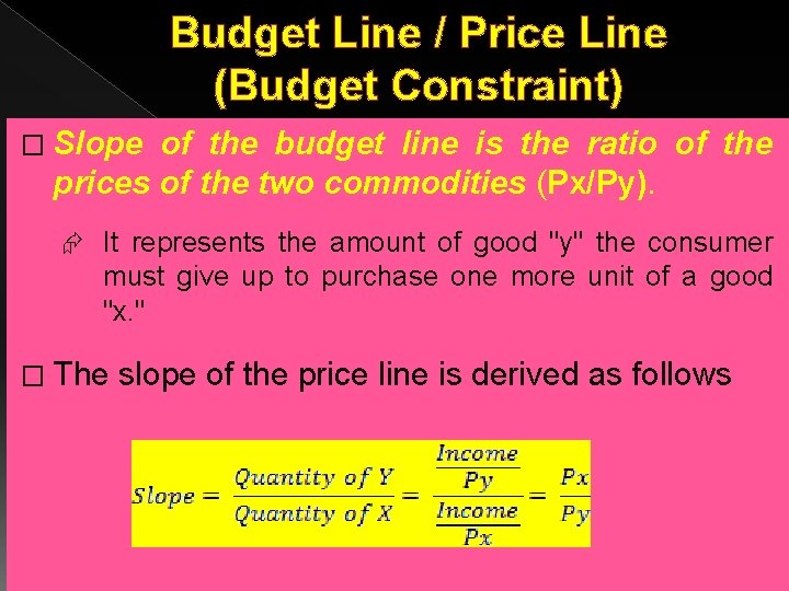
Budget Line / Price Line (Budget Constraint) � Slope of the budget line is the ratio of the prices of the two commodities (Px/Py). It represents the amount of good "y" the consumer must give up to purchase one more unit of a good "x. " � The slope of the price line is derived as follows

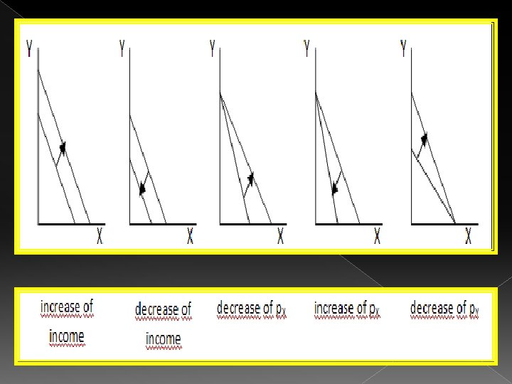
Change in Budget/Price Line � Budget line is drawn with the assumptions of constant income of consumer and constant prices of the commodities. � A new budget line would have to be drawn if either (a) Income of the consumer changes, (b) Price of the commodity changes.

Change in Budget/Price Line � Prices remaining the same, change in income, causes a parallel shift in the BL. If income increases, the BL shifts parallel outwards, to the right, slope remaining constant. If income decreases, the BL shifts parallel inwards to the left, slope remaining constant.

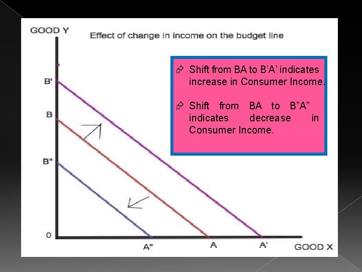
Shift from BA to B’A’ indicates increase in Consumer Income. Shift from BA to B”A” indicates decrease in Consumer Income.

Change in Budget/Price Line � Change in the price of a good, income remaining the same, causes the budget line to rotate on its axis. � If price of X falls, price line rotates outwards, slope decreases and vice versa. � If price of Y falls, price line rotates outwards, slope decreases and vice versa.

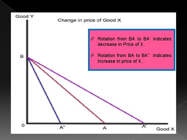
Rotation from BA to BA’ indicates decrease in Price of X. Rotation from BA to BA” indicates increase in price of X.

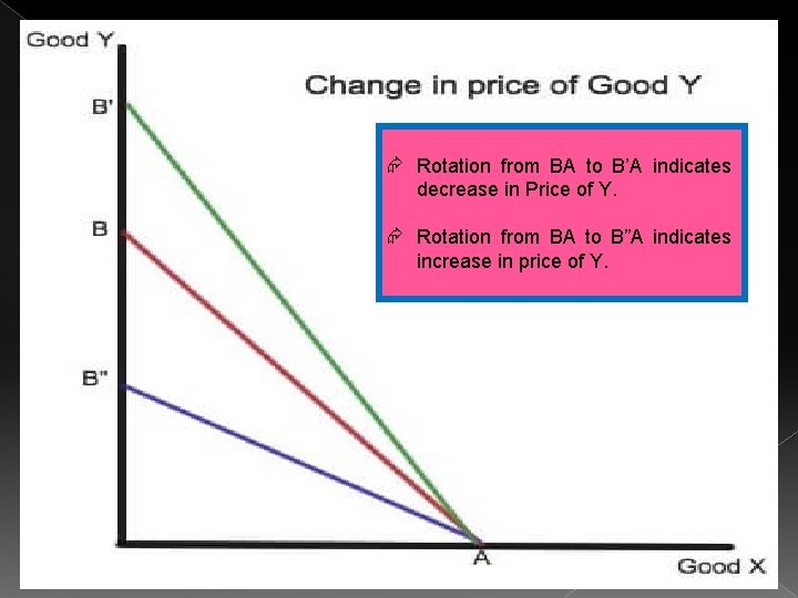
Rotation from BA to B’A indicates decrease in Price of Y. Rotation from BA to B”A indicates increase in price of Y.

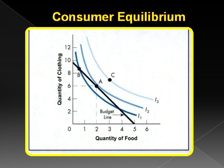
Consumer Equilibrium � A consumer is in equilibrium when the consumer maximizes his/her total utility or satisfaction subject to the income and price constraints. � It can be illustrated by superimposing the indifference map on the budget line. � Indifference map shows the preferences of consumer and the budget line shows the income and price constraints by the consumer.

Consumer Equilibrium � A consumer is in equilibrium when the budget line is tangent to the highest possible indifference curve. � At the point of tangency, the slope of the indifference curve is equal to the slope of the budget line.

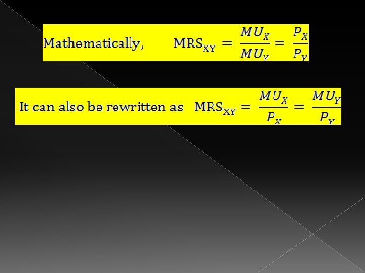
Consumer Equilibrium � The slope of the indifference curve measures the marginal rate of substitution and the slope of the budget line is the price ratio of the two goods. � Thus the equilibrium of the consumer is at the point of tangency of an indifference curve with the budget line. � This implies that the marginal rate of substitution of the two goods is equal to the ratio of their prices.

Consumer Equilibrium

Effect of Change in Income on Consumer Equilibrium � If income decreases, the BL shifts inwards towards the origin and the consumer will move on to equilibrium on a lower indifference curve. � If income increases, the BL shifts outwards and the consumer will move on to equilibrium on a higher indifference curve.

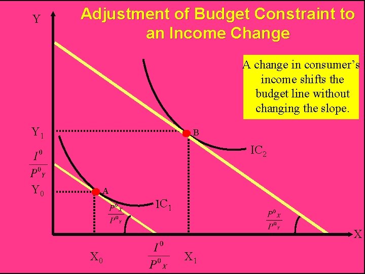
Y Adjustment of Budget Constraint to an Income Change A change in consumer’s income shifts the budget line without changing the slope. Y 1 B IC 2 Y 0 A IC 1 X X 0 X 1

Effect of Change in Price on Consumer Equilibrium � If price of commodity X falls, the price line rotates outwards, to the right and the consumer will move on to equilibrium on a higher indifference curve. � If it increases, the price line rotates inwards and the consumer will move on to equilibrium on a lower indifference curve.

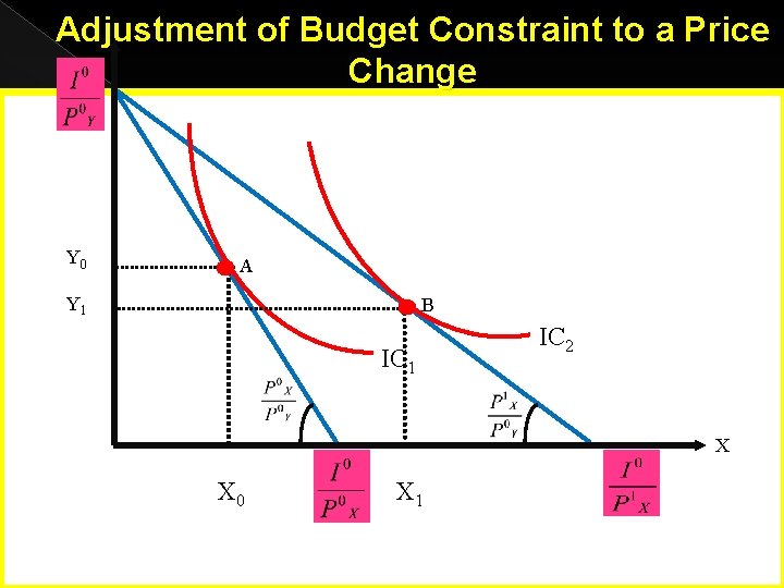
Adjustment of Budget Constraint to a Price Y Change Y 0 A Y 1 B IC 1 IC 2 X X 0 X 1

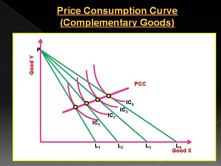
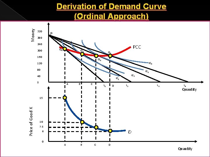
Price Consumption Curve (Complementary Goods) Good Y P PCC IC 4 IC 2 IC 3 IC 1 L 2 L 3 L 4 Good X

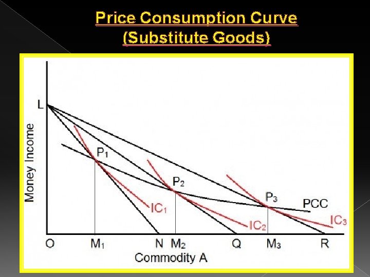
Price Consumption Curve (Substitute Goods)

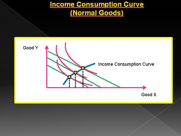
Income Consumption Curve (Normal Goods) Good Y Income Consumption Curve Good X

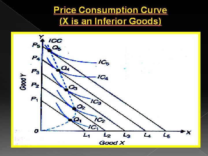
Price Consumption Curve (X is an Inferior Goods)

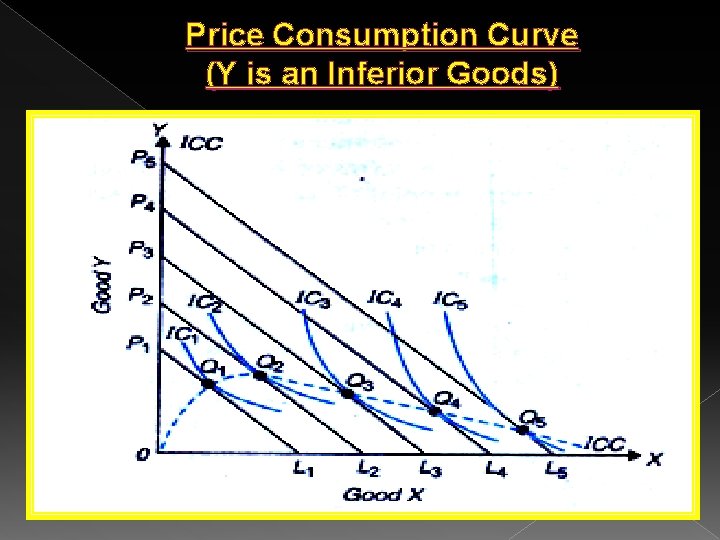
Price Consumption Curve (Y is an Inferior Goods)

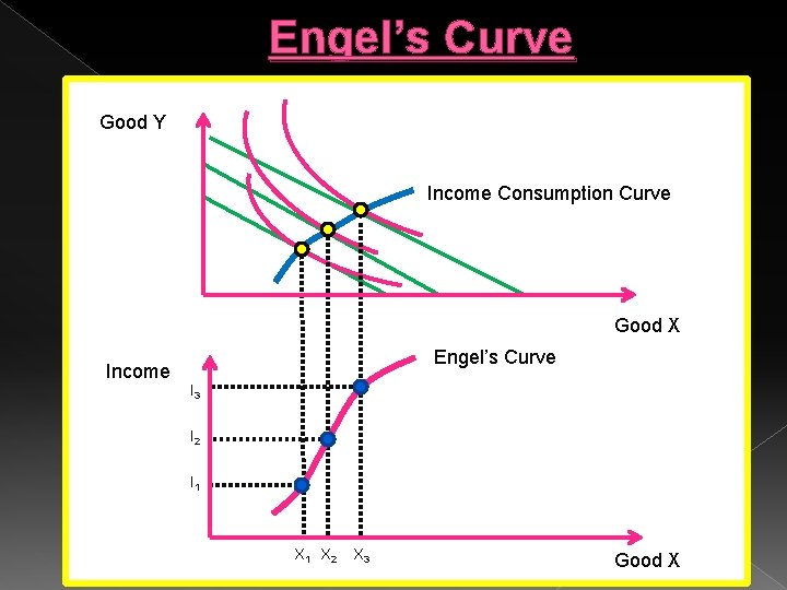
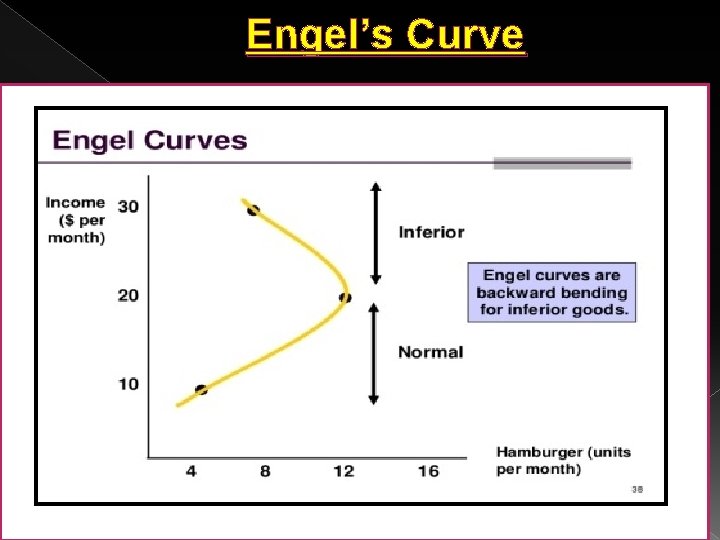
Engel’s Curve Good Y Income Consumption Curve Good X Income Engel’s Curve I 3 I 2 I 1 X 2 X 3 Good X

Engel’s Curve

Income (Y) Engel’s Curve Normal Good Y 1 Y Inferior Good Q 3 Q Q 1 Quantity

Income (Y) Engel’s Curve Normal Good Y 1 Y Inferior Good Q 3 Q Q 1 Quantity

Money Derivation of Demand Curve (Ordinal Approach) 320 280 P 240 200 Q 1 PCC Q 2 Q 4 160 Q 3 120 IC 4 80 40 IC 2 IC 1 0 A B C L 1 D L 2 IC 3 L 4 Quantity Price of Good X 15 10 7. 5 6 0 D A B C D Quantity

Price, Income and Substitution Effects (Hicks and Slutsky) � PRICE EFFECT = INCOME EFFECT + SUBSTITUTION EFFECT INCOME EFFECT � In a two-commodity model, suppose a consumer’s money income is constant. � Assume that the price of one commodity falls. � This results in an increase in the consumer’s real income, which raises his purchasing power. � Due to an increase in the real income, the consumer is now able to purchase more quantity of commodities. This is known as Income Effect. � Income effect refers to the change in quantity demanded of a good due to changes in the real income of the consumer assuming that the tastes and preferences of the consumer remains unchanged.

Price, Income and Substitution Effects (Hicks and Slutsky) � PRICE EFFECT = INCOME EFFECT + SUBSTITUTION EFFECT � Consider a two-commodity model for simplicity. � When the price of one commodity falls, the consumer substitutes the cheaper commodity for the costlier commodity. � This is known as Substitution Effect. � It is the change in consumption pattern brought about by a change in relative price of a good.

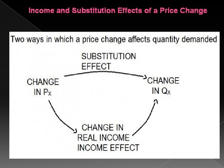
Income and Substitution Effects of a Price Change

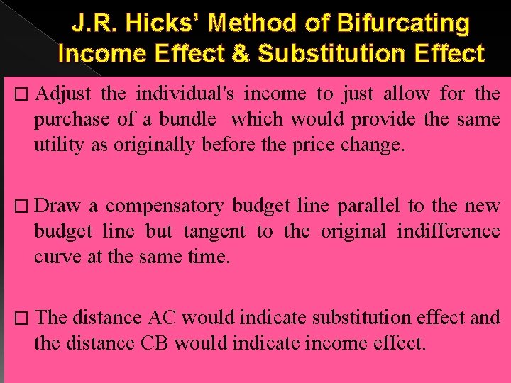
J. R. Hicks’ Method of Bifurcating Income Effect & Substitution Effect � Adjust the individual's income to just allow for the purchase of a bundle which would provide the same utility as originally before the price change. � Draw a compensatory budget line parallel to the new budget line but tangent to the original indifference curve at the same time. � The distance AC would indicate substitution effect and the distance CB would indicate income effect.

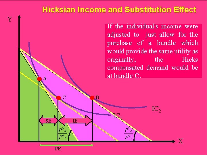
Hicksian Income and Substitution Effect Y If the individual's income were adjusted to just allow for the purchase of a bundle which would provide the same utility as originally, the Hicks compensated demand would be at bundle C. A C SE B IE IC 1 IC 2 X PE

Slutsky’s Method of Separating Income Effect & Substitution Effect � Reduce the consumer’s money income in such a way that he returns to his original equilibrium point even after the price change. � Draw an imaginary budget line, which passes through the original equilibrium point but parallel to the new budget line. � The distance AC would indicate substitution effect and the distance CB would indicate income effect.

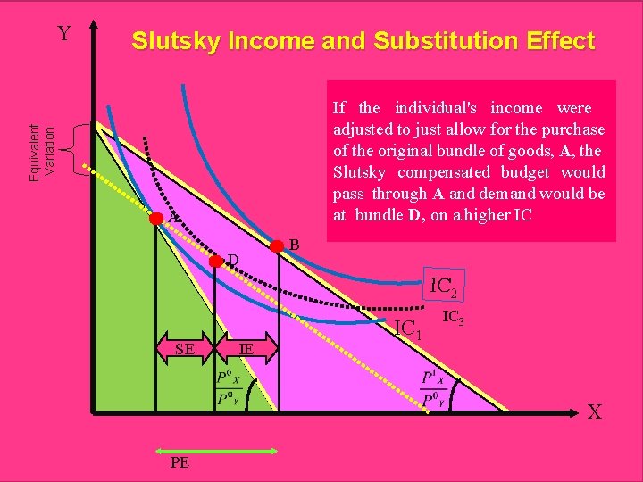
Slutsky Income and Substitution Effect If the individual's income were adjusted to just allow for the purchase of the original bundle of goods, A, the Slutsky compensated budget would pass through A and demand would be at bundle D, on a higher IC Equivalent Variation Y A D B IC 2 SE IE IC 1 IC 3 X PE

Consumer’s Surplus - Hicksian Method (Ordinal Measurement) � Consumers’ surplus is defined as the difference between the price that the consumer is prepared to pay and the price that is actually paid for a commodity. � In Hicksian analysis consumers’ surplus is shown as the vertical distance between indifference curves.

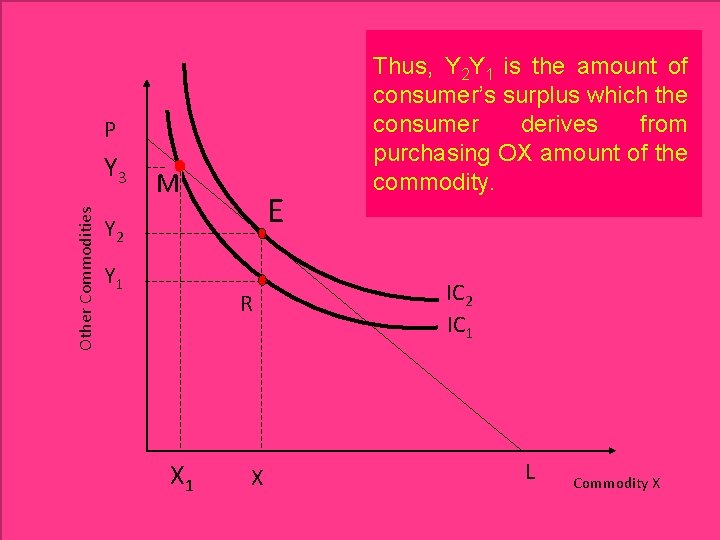
P Other Commodities Y 3 M E Y 2 Y 1 R X 1 X Thus, Y 2 Y 1 is the amount of consumer’s surplus which the consumer derives from purchasing OX amount of the commodity. IC 2 IC 1 L Commodity X

Y Normal, Inferior and Giffen Goods – When Price Falls Giffen Inferior Normal BG BI A C B U 0 PE IE X 0 SE X 1 SE X 2 PE SE IE IE X 3 X

Revealed Preference Analysis

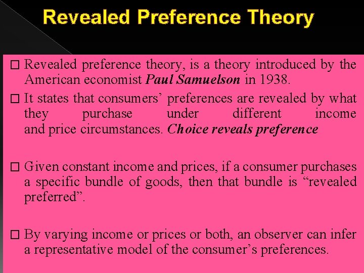
Revealed Preference Theory Revealed preference theory, is a theory introduced by the American economist Paul Samuelson in 1938. � It states that consumers’ preferences are revealed by what they purchase under different income and price circumstances. Choice reveals preference � � Given constant income and prices, if a consumer purchases a specific bundle of goods, then that bundle is “revealed preferred”. � By varying income or prices or both, an observer can infer a representative model of the consumer’s preferences.

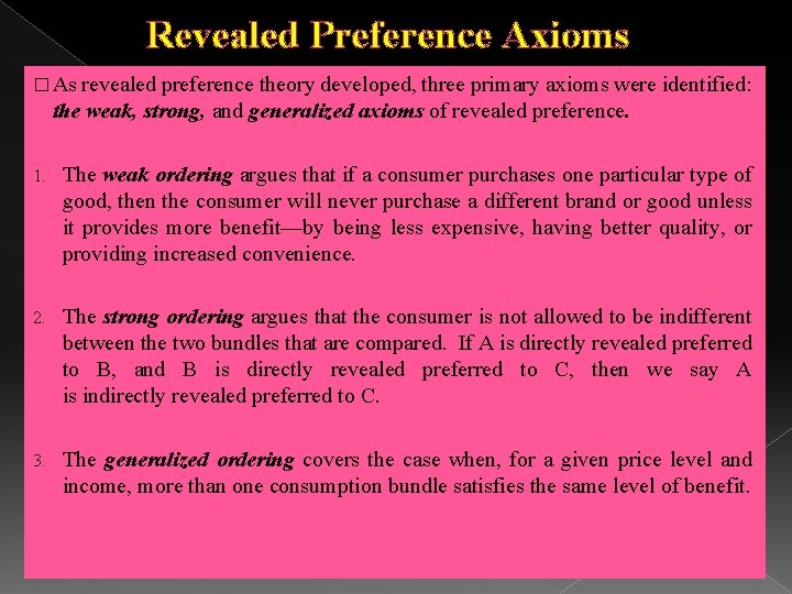
Revealed Preference Axioms � As revealed preference theory developed, three primary axioms were identified: the weak, strong, and generalized axioms of revealed preference. 1. The weak ordering argues that if a consumer purchases one particular type of good, then the consumer will never purchase a different brand or good unless it provides more benefit—by being less expensive, having better quality, or providing increased convenience. 2. The strong ordering argues that the consumer is not allowed to be indifferent between the two bundles that are compared. If A is directly revealed preferred to B, and B is directly revealed preferred to C, then we say A is indirectly revealed preferred to C. 3. The generalized ordering covers the case when, for a given price level and income, more than one consumption bundle satisfies the same level of benefit.

Assumptions 1. 2. Consumer is assumed to behave rationally. Consumer’s tastes do not change. 3. The consumer behave consistently i. e. if he chooses bundle A in a situation in which bundle B was also available to him, he will not choose B in any other situation in which A is also available. 4. Transitivity: If in any particular situation A ˃ B and B ˃ C then A ˃ C. 5. Strong Ordering: The consumer can clearly arrange in order of preference each item in a bundle. 6. Consumer chooses only one combination at a time. 7. He prefers a combination of more goods to less in any situation. 8. Income elasticity of demand is positive i. e. , more commodity is demanded when income increases, and vice versa.

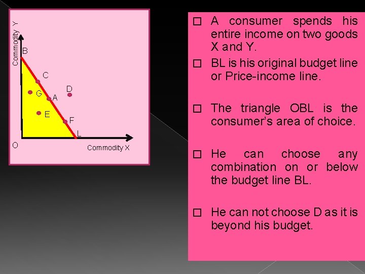
Commodity Y A consumer spends his entire income on two goods X and Y. � BL is his original budget line or Price-income line. � B C G A E D � The triangle OBL is the consumer’s area of choice. � He can choose any combination on or below the budget line BL. � He can not choose D as it is beyond his budget. F L O Commodity X

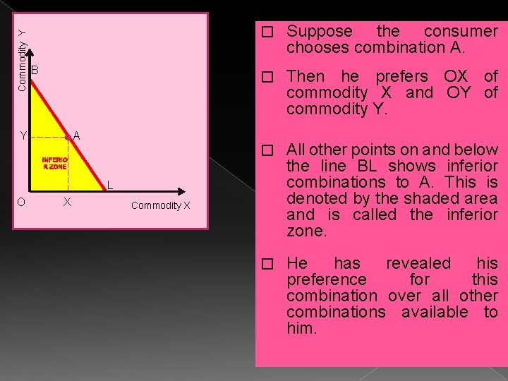
Commodity Y B � Suppose the consumer chooses combination A. � Then he prefers OX of commodity X and OY of commodity Y. � All other points on and below the line BL shows inferior combinations to A. This is denoted by the shaded area and is called the inferior zone. � He has revealed his preference for this combination over all other combinations available to him. A Y INFERIO R ZONE L O X Commodity X

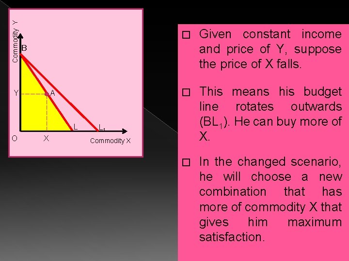
Commodity Y Given constant income and price of Y, suppose the price of X falls. � This means his budget line rotates outwards (BL 1). He can buy more of X. � In the changed scenario, he will choose a new combination that has more of commodity X that gives him maximum satisfaction. B A Y L O � X L 1 Commodity X

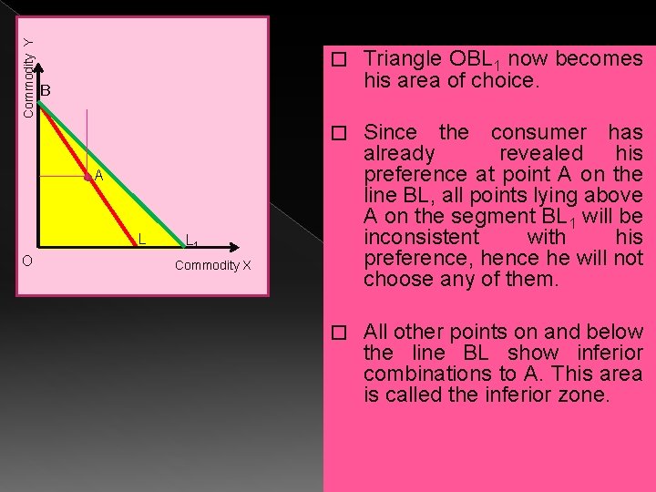
Commodity Y � Triangle OBL 1 now becomes his area of choice. � Since the consumer has already revealed his preference at point A on the line BL, all points lying above A on the segment BL 1 will be inconsistent with his preference, hence he will not choose any of them. � All other points on and below the line BL show inferior combinations to A. This area is called the inferior zone. B A L O L 1 Commodity X

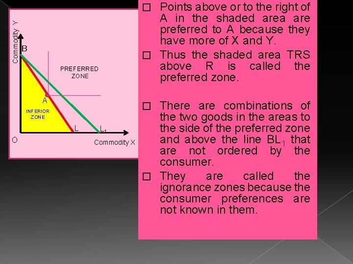
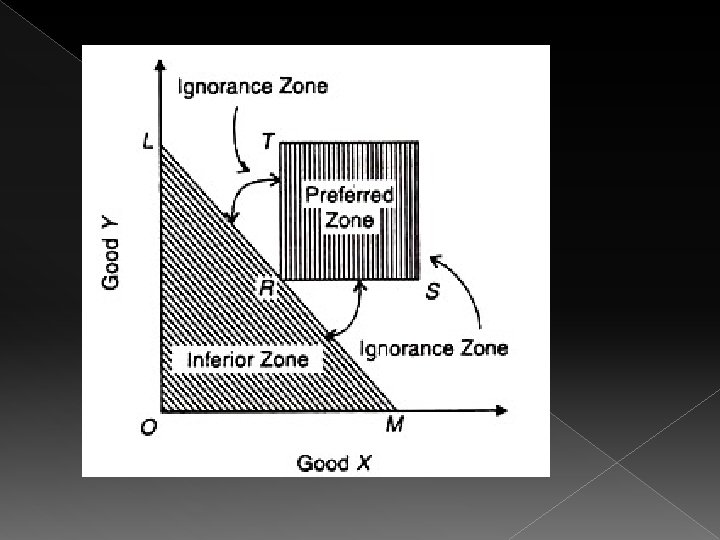
Points above or to the right of A in the shaded area are preferred to A because they have more of X and Y. � Thus the shaded area TRS above R is called the preferred zone. Commodity Y � B PREFERRED ZONE A L O There are combinations of the two goods in the areas to the side of the preferred zone and above the line BL 1 that are not ordered by the consumer. � They are called the ignorance zones because the consumer preferences are not known in them. � INFERIOR ZONE L 1 Commodity X