Module 9 3 Random Numbers from Various Distributions

Introduction • Monte Carlo simulations are important tools in scientific work and yield solutions to problems unobtainable by other means. Moreover, where alternative solutions are possible, such simulations often provide greater precision for the same computer cost. • A Monte Carlo simulation requires the use of unbiased random numbers.

Distribution of numbers • Description of portion of times each possible outcome or each possible range of outcomes occurs on the average over many trials. • The distribution that a simulation requires depends on the problem.

Uniform distribution • Just as likely to return value in any interval • In list of many random numbers, on the average each interval contains same number of generated values

Uniform distribution The relative frequency of each interval is about the same ≈ 0. 1.

Discrete distribution • Distribution with discrete values • Probability function (or density function or probability density function) • Returns probability of occurrence of particular argument value. For example, roll a fair die, P(X = x) = 1/6 where x = 1, 2, 3, 4, 5, 6.

Uniform Discrete Distribution • To Generate Random Numbers in Discrete Distribution with Equal Probabilities for Each of n Events • Generate uniform random integer from a sequence of n integers, where each integer corresponds to an event. For example, a simulation of flipping a coin: head = 0 and 1 = tail

Discrete Distribution To generate random numbers in discrete distribution with probabilities p 1, p 2, …, pn for events e 1, e 2, …, en, respectively, where p 1 + p 2 + … + pn = 1 Generate rand, uniform random floating point number in [0, 1) If rand < p 1, then return e 1 else if rand < p 1 + p 2, then return e 2 … else if rand < p 1 + p 2 + … + pn - 1, then return en - 1 else return en

Continuous distribution • Distribution with continuous values • Probability function (or density function or probability density function) • Indicates probability that given outcome falls inside specific range of values

Normal or Gaussian distribution • Probability density function, where µ is mean and σ is standard deviation: 68. 3% of the values in (μ – σ, μ – σ) 95. 5% of the values in (μ – 2σ, μ – 2σ) 99. 7% of the values in (μ – 3σ, μ – 3σ)

Box-Muller-Gauss Method •

Box-Muller-Gauss Method

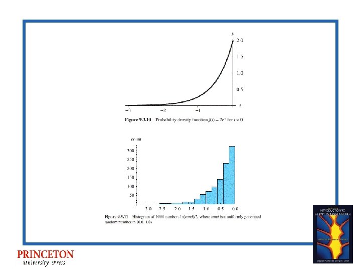
Exponential Distributions • Probability density functions: • f(t) = |r|ert with r < 0 and t > 0 or f(t) = |r|ert with r > 0 and t < 0 • Graph of f(t) = 2 e-2 t

Exponential Method • For probability density function f(t)= |r|ert with r < 0 and t > 0 or f(t) = |r|ert with r > 0 and t < 0 • Compute ln(rand)/r, where rand = a uniform random number in [0. 0, 1. 0)

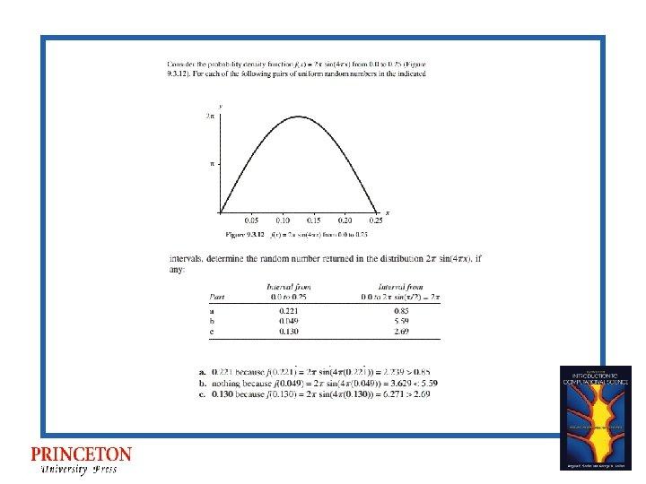
Rejection Method - When other methods do not apply • For random numbers in interval [a, b) for distribution f(x) • If f(rand. Interval) > rand. Upper. Bound, then return rand. Interval, where • rand. Interval - uniform random number in interval [a, b) • rand. Upper. Bound - uniform random number in [0, upper bound for f) • else repeat the process