Module 6 Introduction to Parallel Processing What is

Module 6 Introduction to Parallel Processing

What is Serial Computing? • Traditionally, software has been written for serial computation: – To be run on a single computer having a single Central Processing Unit (CPU); – A problem is broken into a discrete series of instructions. – Instructions are executed one after another. – Only one instruction may execute at any moment in time.

Serial Computing

Example

Parallel Computing • Parallel computing is the simultaneous use of multiple compute resources to solve a computational problem. • How? – To be run using multiple processors – A problem is broken into discrete parts that can be solved concurrently – Each part is further broken down to a series of instructions – Instructions from each part execute simultaneously on different processors – An overall control/coordination mechanism is employed

Parallel Computing

Example

Why Use Parallel Computing? • SAVE TIME AND/OR MONEY: • Assigning more resources at a task will shorten its time to completion, with potential cost savings. • Parallel computers can be built from cheap, commodity components.

Why Use Parallel Computing? • SOLVE LARGER / MORE COMPLEX PROBLEMS • Solves problems that are so large and/or complex that it is impractical to solve them on a single computer. • Example: Web search engines/databases processing millions of transactions per second

Why Use Parallel Computing? • PROVIDE CONCURRENCY: Multiple compute resources can do many things simultaneously. • Example: the Access Grid provides a global collaboration network where people from around the world can meet and conduct work "virtually".

Why Use Parallel Computing? • TAKE ADVANTAGE OF NON-LOCAL RESOURCES: Using compute resources on a wide area network, or even the Internet when local compute resources are scarce or insufficient. • Example: SETI@home : over 1. 3 million users, 3. 4 million computers in nearly every country in the world.

Flynn’s Classification of Parallel Processors • classified along 2 independent dimensions of Instruction Stream and Data Stream. Each with two possible states: Single or Multiple.

Single Instruction, Single Data (SISD) • A serial (non-parallel) computer • Single Instruction: Only one instruction stream is being acted on by the CPU during any one clock cycle • Single Data: Only one data stream is being used as input during any one clock cycle • Examples: older generation mainframes, minicomputers, workstations and single processor/core PCs.

SISD

Examples

Single Instruction, Multiple Data (SIMD) • A type of parallel computer • Single Instruction: All processing units execute the same instruction at any given clock cycle • Multiple Data: Each processing unit can operate on a different data element • Best suited for specialized problems characterized by a high degree of regularity: e. g. graphics/image processing. • Two varieties: Processor Arrays and Vector Pipelines

Array Processor

Example

Vector Processor

Examples

Multiple Instruction, Single Data (MISD) • A type of parallel computer • Multiple Instruction: Each processing unit operates on the data independently via separate instruction streams. • Single Data: A single data stream is fed into multiple processing units. • Few actual examples • Some conceivable uses might be: – multiple frequency filters operating on a single signal stream – multiple cryptography algorithms attempting to crack a single coded message.

Multiple Instruction, Single Data (MISD)

Multiple Instruction, Single Data (MISD)

Multiple Instruction, Multiple Data (MIMD) • A type of parallel computer • Multiple Instruction: Every processor may be executing a different instruction stream • Multiple Data: Every processor may be working with a different data stream • Most modern supercomputers fall into this category.

Multiple Instruction, Multiple Data (MIMD)

Examples

Parallel Organizations • Control Unit (CU) provides Instruction Stream (IS) • Processing Unit (PU) operates on Data Stream (DS) from Memory Unit (MU)

SISD SIMD

MIMD • MIMD can be further subdivided into two by the means in which the processor’s communicate 1. Tightly Coupled : Shared Memory 2. Loosely Coupled : Distributed memory

MIMD : Shared Memory

MIMD : Shared Memory • In this model, tasks share a common address space. • Mechanisms such as locks may be used to control access to the shared memory. • Advantage : the notion of data "ownership" is lacking, thus program development can often be simplified. • Disadvantage: controlling data locality is hard to understand may be beyond the control of the average user.

MIMD: Distributed Memory

MIMD: Distributed Memory • A set of tasks that use their own local memory during computation. • Tasks exchange data through communications by sending and receiving messages. • Data transfer requires cooperative operations to be performed by each process. For example, a send operation must have a matching receive operation. • MPI(Message Passing Interface): standard interface

MIMD: Distributed Memory

Pipelining • It is a technique of decomposing a sequential process into sub-operations with each subprocess being executed in a special dedicated segment that operates concurrently with all other segments • It improves processor performance by overlapping the execution of multiple instructions

Example

Pipelining: Its Natural! • Laundry Example • Ann, Brian, Cathy, Dave each have one load of clothes to wash, dry, and fold • Washer takes 30 minutes • Dryer takes 40 minutes • Folder takes 20 minutes A B C D

Sequential Laundry 6 PM 7 8 9 10 11 Midnight Time 30 40 20 T a s k O r d e r A B C D • Sequential laundry takes 6 hours for 4 loads • If they learned pipelining, how long would laundry take?

Pipelined Laundry Start work ASAP 6 PM 7 8 9 10 11 Time 30 40 T a s k O r d e r 40 40 40 20 A B C D • Pipelined laundry takes 3. 5 hours for 4 loads Midnight

Observations on Pipeline Processing • It works well if time taken by each stage is nearly the same – If this time is T seconds, then the pipeline produces output at every T seconds – If time taken by each stage varies, then the slower stage becomes a bottleneck in the progress

Pipelined Laundry 6 PM 30 A B C D 7 30 30 8 30 30 30 • Suppose each stage Time takes 30 minutes 9 PM 30 30 30 • Time to wash, dry, and fold one load is still the same (90 minutes) • Then the work will get over in 3 hours

Pipelined Laundry 6 PM 7 8 9 10 11 Time 30 40 T a s k O r d e r 40 40 40 20 A B C D • Here 40 minutes takes over the pipeline cycle Midnight

Instruction Pipelining

Instruction Pipelining • Consider subdividing instruction processing into 2 stages: fetch and execute • While second stage executes instruction, the first stage fetches and buffers next instruction (instruction prefetch) • Advantage: doubles execution rate • Disadvantage : – Execution time is more than fetch time – Conditional branch : Fetch stage have to wait for address from execute stage.

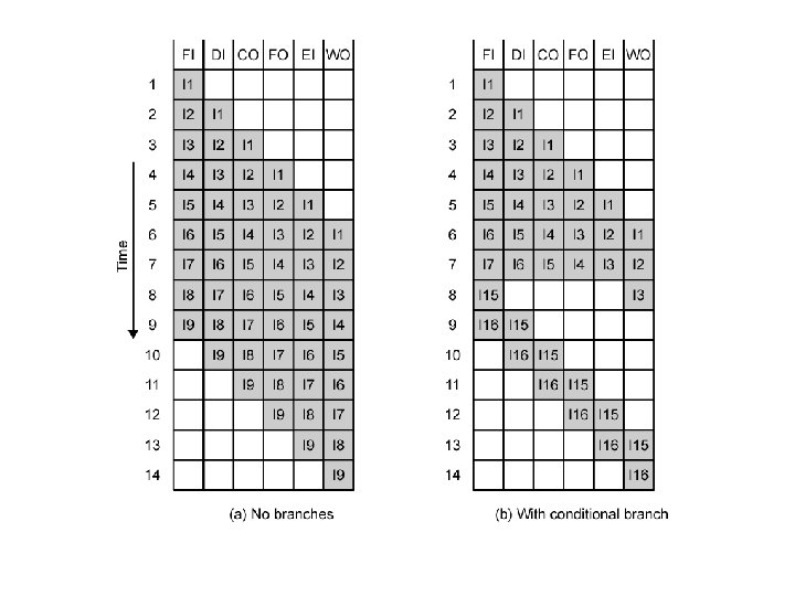
Instruction Pipelining • To gain further speedup, the pipeline must have more stages. Thus instruction processing is divided into following 6 stages: – Fetch Instruction(FI): Read next instruction to buffer – Decode Instruction(DI): Determine opcode and operand specifiers – Calculate Operands (CO): Calculate address of source operands – Fetch Operands(FO): Fetch operands from memory – Execute Instructions(EI): Perform the indicated operation – Write Operand(WO): Store result in memory

State Diagram for Instruction Pipelining

Instruction Pipelining • A six stage pipeline can reduce execution time from 54 time units to 14 time units

Limitations of 6 -stage pipeline • Assumes that each instruction goes thru all 6 stages. This will not always true. E. g. LOAD does not require WO stage. • Assumes that all stages can be performed in parallel and there are no memory conflicts. However FI, FO and WO can occur simultaneously and most memory systems does not permit that.

Limitations of 6 -stage pipeline • If six stages are not of equal duration, there will be some waiting time involved at various pipeline stages. • The conditional branch instruction and interrupt can invalidate several instruction fetches. • Register conflict and Memory conflict

Pipeline Hazards • A pipeline hazard occurs when the pipeline must stall because some conditions do not permit continued execution. • It is also referred to as a pipeline bubble. • There are three types of hazards: resource, data and control.

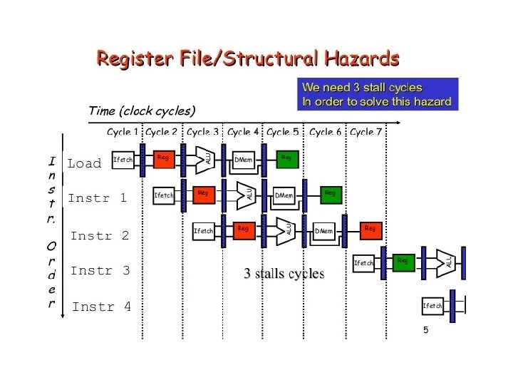
Resource Hazard • A resource hazard occurs when two or more instructions in the pipeline need the same resource.

Data Hazards • A data hazard occurs when there is a conflict in the access of an operand location. • Hazards are caused by resource usage conflicts among various instructions • They are triggered by inter-instruction dependencies

Hazard Detection and Resolution Terminologies: • Resource Objects: set of working registers, memory locations and special flags • Data Objects: Content of resource objects • Each Instruction can be considered as a mapping from a set of data objects to a set of data objects.

Hazard Detection and Resolution • Domain D(I) : set of resource of objects whose data objects may affect the execution of instruction I. (e. g. Source Registers) • Range R(I): set of resource objects whose data objects may be modified by the execution of instruction I. (e. g. Destination Register) • Instruction reads from its domain and writes in its range

Hazard Detection and Resolution • Consider execution of instructions I and J, and J appears immediately after I. • There are 3 types of data dependent hazards: 1. RAW (Read After Write) 2. WAW(Write After Write) 3. WAR (Write After Read)

RAW (Read After Write) • The necessary condition for this hazard is

RAW (Read After Write) • Example: I 1 : LOAD r 1, a I 2 : ADD r 2, r 1 • I 2 cannot be correctly executed until r 1 is loaded • Thus I 2 is RAW dependent on I 1

WAW(Write After Write) • The necessary condition is

WAW(Write After Write) • Example I 1 : MUL r 1, r 2 I 2 : ADD r 1, r 4 • Here I 1 and I 2 writes to same destination and hence they are said to be WAW dependent.

WAR(Write After Read) • The necessary condition is

WAR(Write After Read) • • Example: I 1 : MUL r 1, r 2 I 2 : ADD r 2, r 3 Here I 2 has r 2 as destination while I 1 uses it as source and hence they are WAR dependent

Hazard Detection and Resolution • Hazards can be detected in fetch stage by comparing domain and range. • Once detected, there are two methods: 1. Generate a warning signal to prevent hazard 2. Allow incoming instruction through pipe and distribute detection to all pipeline stages.

Control Hazards • Instructions that disrupt the sequential flow of control present problems for pipelines. • The following types of instructions can introduce control hazards: – Unconditional branches. – Conditional branches. – Indirect branches. – Procedure calls. – Procedure returns.

Solutions for Control Hazards • The following are solutions that have been proposed for mitigating control hazards: – Pipeline stall cycles: Freeze the pipeline until the branch outcome and target are known, then proceed with fetch. – Branch delay slots: The compiler must fill these branch delay slots with useful instructions or NOPs – Branch prediction.