Module 4 Community structure and assembly Class Day
 Topic Intro,")
Module 4: Community structure and assembly Class Day 1 (Thu Nov 1) Topic Intro, definitions, some history. Messing around with a simple dataset in R. Day 2 (Tue Nov 6) Day 3 (Thu Nov 8) Paper discussion 1: Niches across scales Chase and Myers (2011) Paper discussion 2: Can we begin to infer Leibold and Mikkelson community assembly processes from (2002) patterns? Day 4 (Tue Nov 13) Paper discussion 3: do communities actually exist? Day 5 (Thu Nov 15) Day 6 (Tue Nov 27) Reading(s) Half the class will read Ricklefs (2008) and half will read Brooker et al. (2009). 5 datasets, 5 groups (TBD). ‘Elements of metacommunity Structure’ approach applied to datasets using R package metacom. Brief group presentations and discussion. Is the world Clementsian/Gleasonian/neutral/other?

Themes of this module § How do we quantify diversity across scales? § What does it tell us about community assembly?

Learning objectives § Understand key foundational ecological concepts § Understand some of the key mechanisms driving community assembly and patterns of diversity across scales § Learn basic R tools for analyzing communities and metacommunities § What is the relationship between pattern and process, and what are limits to this relationship?

Some key concepts The niche Environmental filtering Competition and competitive exclusion Succession Dispersal limitation Community assembly Metacommunity Deterministic vs. stochastic processes Niche vs. neutral processes

NICHES

The niche concept https: //www. merriam-webster. com
 § Eltonian niche (Elton")
The niche concept and competition § Grinnellian niche (Grinnell 1917) § Eltonian niche (Elton 1927) § Niche is “n-dimensional”, maps population dynamics onto environmental space (Hutchinson 1957) § Competitive exclusion principle (Hardin 1960) § Mac. Arthur and Levins (1967): limiting similarity
: fundamental niche concept Red oak Spring temperature Tradeoff axis Species turnover occurs")
Hutchinson (1957): fundamental niche concept Red oak Spring temperature Tradeoff axis Species turnover occurs across this axis Beech Precipitation Modified from Clark et al. (2011)
: fundamental niche concept The two species can co-occur in this parameter space,")
Hutchinson (1957): fundamental niche concept The two species can co-occur in this parameter space, and compete for resources Spring temperature Red oak Beech Precipitation Modified from Clark et al. (2011)
: fundamental niche concept Spring temperature Sp A Sp B Sp C No")
Hutchinson (1957): fundamental niche concept Spring temperature Sp A Sp B Sp C No turnover in this case; there is nestedness across space Why doesn’t Sp C occur here? Biotic interaction with Sp A or B or ‘environmental filtering? ’ Precipitation Fundamental vs. realized niche

Species distributions form successive Gaussian envelopes along environmental gradients A B CD Environmental gradient Whittaker (1965, 1967)

COMPETITION

Resource consumption often leads to resource depletion – AND COMPETITION § The ability of a species to maintain itself in a community is determined by the limiting resource level (R*) that results in zero net population growth (ZNPG). § This depends on the supply and consumption rates of the resource and the reproduction and mortality rates of the consumer species. Image/fig from Cain et al. (2014) Tilman (1980); Tilman et al. (1981)

Two species may have different R* values corresponding to their respective ZNPG states Image/fig from Cain et al. (2014)

In competition, Synedra has a lower R*, and outcompetes Asterionella R* represents the level of the resource that will allow a species to persist If R* is low, the resource is being used efficiently What can we say about the niches of each of these species? Image/fig from Cain et al. (2014)

What happens when von Liebig's Law of there are multiple Minimum: yield is proportional resources? to the amount of the most limiting nutrient in the soil A population will grow until one resource becomes limiting for further growth Organisms need many resources – but von Liebig suggested that at any given time only one is limiting http: //corn. osu. edu/ Image/fig from Cain et al. (2014)

LOCAL COEXISTENCE

Tilman’s R* provides a mechanism for understanding competitive exclusion and coexistence in terms of population dynamics Species A Growth rate m. A Species B Two species, one resource – who wins? m. B R*A Resource R What happens when there are two potentially limiting resources?

Two species, two resources Consumption vectors Species B Resource 2 Species A 1 2 3 4 5 Species B 6 Species A Resource 1 Only a resource supply in zone 4 will lead to the coexistence point, but this shows that conditions exist that allow coexistence

Tilman showed experimentally that certain combinations of resource ratios and nutrient supply rates allowed stable coexistence between two diatom species Image/fig from Cain et al. (2014)

All plants need similar resources – how do so many species coexist?

At any given point in space, two species that don’t occupy the same niche can coexist when there are two limiting resources It follows that if there are n limiting resources, n species can theoretically coexist BUT – there are only so many resources… Hutchinson (1961), in “The paradox of the plankton” asked, how do n+ species coexist on n resources?
 expanded the two-species case to incorporate many species")
Tilman (1988) expanded the two-species case to incorporate many species

One way -> if there is spatial variation in resource supply rates If the environment is homogeneous, we can think of the supply point as exactly that – a point, and only two species coexist Tilman (1988)

But if we have substantial spatial heterogeneity in supply rates and resource ratios, many species can coexist Tilman (1988)
, Panama Soil N")
Another example: soil N and P in Barro Colorado Island (BCI), Panama Soil N Soil P http: //www. life. illinois. edu/
")
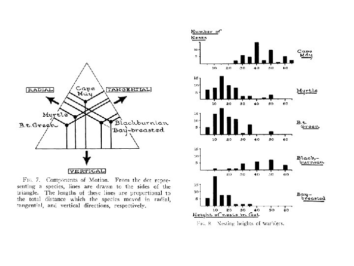
Macarthur’s warblers and niche partitioning Myrtle warbler Black-throated green warbler Mac. Arthur (1967)

To sum up: some mechanisms that may explain local species richness: § Resource ratios § Hutchinson (1961): Non-equilibrium § Spatial heterogeneity in resource ratios § Niche partitioning § Others?

SUCCESSION
 -> succession in Lake Michigan dune communities Clements")
Clementsian vs. Gleasonian succession Cowles (1899) -> succession in Lake Michigan dune communities Clements (1916) -> communities as “superorganisms”, succession as analogous to development – climax state Gleason (1926) -> “individualistic model”: species interact during succession, but not in an integrated fashion
 and the Institute Woods Horn (1975)")
Horn (1975) and the Institute Woods Horn (1975)

Horn’s table in cartoon form… Sassafras Red maple Beech

A simulation of succession based on Horn’s overstory/understory data
 Disturbance creates colonization opportunities Facilitation: first species")
Models of succession (Connel and Slatyer 1977) Disturbance creates colonization opportunities Facilitation: first species change conditions to allow later species to colonize. Implies high level of community integration. Tolerance: later species take time to disperse, grow, and establish. They grow despite the presence of early-successional species, and eventually outcompete them. Climax Inhibition: earlysuccessional species inhibit colonization by all others. Late successional species are those that are able to survive better.

Our focus so far: LOCAL coexistence of things that are interacting with each other Let’s shift to larger scales

Diversity across scales Spatial scale Regional scale γ diversity Turnover β diversity Community scale α diversity Image/fig from Cain et al. (2014)

A cartoonish, non-quantitative example Plot 1 B AAB B A B AB C A D B A D D C Plot 2 D CC D D C Example 1 Low α, High β B B C A D AB C C D Example 2 High α, Low β Can we infer the mechanisms that gave rise to these patterns simply by analyzing the patterns themselves?

DISPERSAL LIMITATION
 Area and distance (≈ isolation)")
Theory of Island Biogeography (Mac. Arthur and Wilson 1967) Area and distance (≈ isolation) influence rates of immigration (recolonization) and extinction Effect of area and distance on New Guinea bird species richness Image/fig from Cain et al. (2014)

Area drives extinction rates and distance drives immigration rates Where the two rates balance out, there is an equilibrium species richness Image/fig from Cain et al. (2014)
 on mangrove islands Image/fig from")
The theory was tested by Simberloff and Wilson (1969) on mangrove islands Image/fig from Cain et al. (2014)
: A unified theory of biogeography and relative species abundance")
Enter Hubbell (1997 and 2001): A unified theory of biogeography and relative species abundance § Focuses on two scales: local community dynamics and regional metacommunity dynamics. Generalization of IB to include speciation § Local communities are ‘saturated’ and no births or immigration occurs until spaces are vacated by deaths § They can be recolonized by reproduction by the local species pool or by immigration from the regional pool § No need for niches – species are identical, wide range of species relative abundance distributions explained by this model, which only has 3 parameters θ, J and m § Dispersal limitation is the key § Dispersal is a random (neutral) process
")
Hubbell (1997)

§ So how do niche principles “scale up”? § According to Hubbell, not very well § Neutral model can explain observed patterns very well – niches and competition not needed § Homogeneous environments can be occupied by diverse communities of effectively identical species (in terms of niches) § Hubbell acknowledges that species do have niches, but they don’t matter at large scales

Going forward § What do neutral and niche models have to say about α and β diversity? § What do patterns of α, β diversity tell us about the mechanisms of community assembly? § Is the world niche or neutral, or some of both? § If species differences matter, are communities Gleasonian or Clementsian?
- Slides: 46