MODULE 3 Module 3 Classification Cross validation and

MODULE 3

Module 3 Classification Cross validation and re-sampling methods K-fold cross validation, Boot strapping Measuring classifier performance- Precision, recall, ROC curves. Bayes Theorem, Bayesian classifier, Maximum Likelihood estimation, Density functions,

Evaluation of classifiers In machine learning, there are several classification algorithms and, given a certain problem, more than one may be applicable. There is a need to examine how we can assess how good a selected algorithm is. Also, we need a method to compare the performance of two or more different classification algorithms. These methods help us choose the right algorithm

Methods of evaluation Need for multiple validation sets Statistical distribution of errors No-free lunch theorem Other factors

Need for multiple validation sets When we apply a classification algorithm in a practical situation, we always do a validation test. We keep a small sample of examples as validation set and the remaining set as the training set. The classifier developed using the training set is applied to the examples in the validation set. Based on the performance on the validation set, the accuracy of the classifier is assessed. But, the performance measure obtained by a single validation set alone does not give a true picture of the performance of a classifier.

Need for multiple validation sets Also these measures alone cannot be meaningfully used to compare two algorithms. This requires us to have different validation sets. Cross-validation in general, and k-fold crossvalidation in particular, are two common method for generating multiple training-validation sets from a given dataset � Sample data repeatedly from same sample- resampling

Statistical distribution of errors We use a classification algorithm on a dataset and generate a classifier. If we do the training once, we have one classifier and one validation error. To average over randomness (in training data, initial weights, etc. ), we use the same algorithm and generate multiple classifiers. We test these classifiers on multiple validation sets and record a sample of validation errors.

Statistical distribution of errors We base our evaluation of the classification algorithm on the statistical distribution of these validation errors. We can use this distribution for assessing the expected error rate of the classification algorithm for that problem, or compare it with the error rate distribution of some other classification algorithm.

No-free lunch theorem Whatever conclusion we draw from our analysis is conditioned on the dataset we are given. We are not comparing classification algorithms in a domain-independent way but on some particular application. We are not saying anything about the expected error -rate of a learning algorithm, or comparing one learning algorithm with another algorithm, in general. Any result we have is only true for the particular application.

No-free lunch theorem There is no such thing as the “best” learning algorithm. For any learning algorithm, there is a dataset where it is very accurate and another dataset where it is very poor. This is called the No Free Lunch Theorem

Other factors Classification algorithms can be compared based not only on error rates but also on several other criteria like the following: training time and space complexity, � testing time and space complexity, � interpretability, namely, whether the method allows knowledge extraction which can be checked and validated by experts, � easy programmability. �

Cross-validation To test the performance of a classifier, we need to have a number of training/validation set pairs from a dataset X. To get them, if the sample X is large enough, we can randomly divide it then divide each part randomly into two and use one half for training and the other half for validation. Unfortunately, datasets are never large enough to do this. So, we use the same data split differently; this is called cross-validation.

Cross-validation is a technique to evaluate predictive models by partitioning the original sample into a training set to train the model, and a test set to evaluate it. The holdout method is the simplest kind of cross validation.

Cross-validation The data set is separated into two sets, called the training set and the testing set. The algorithm fits a function using the training set only. Then the function is used to predict the output values for the data in the testing set (it has never seen these output values before). The errors it makes are used to evaluate the

K-fold cross-validation In K-fold cross-validation, the dataset X is divided randomly into K equal-sized parts, Xi , i = 1, . . . , K. To generate each pair, we keep one of the K parts out as the validation set Vi , and combine the remaining K − 1 parts to form the training set Ti. Doing this K times, each time leaving out another one of the K parts out, we get K pairs (Vi , Ti): V 1 = X 1, T 1 = X 2 ∪ X 3 ∪. . . ∪ K X V 2 = X 2, T 2 = X 1 ∪ X 3 ∪. . . ∪ K X V K = X K, TK = X 1 ∪ X 2 ∪. . . ∪ K-1 X

K-fold cross-validation There are two problems with this: � To keep the training set large, we allow validation sets that are small. � The training sets overlap considerably, namely, any two training sets share K − 2 parts. K is typically 10 or 30. � As K increases, the percentage of training instances increases and we get more robust estimators, but the validation set becomes smaller. � Furthermore, there is the cost of training the classifier K times, which increases as K is increased.

Leave-one-out cross-validation An extreme case of K-fold cross-validation is leave-one-out where given a dataset of N instances, only one instance is left out as the validation set and training uses the remaining N − 1 instances. We then get N separate pairs by leaving out a different instance at each iteration. This is typically used in applications such as medical diagnosis, where labeled data is hard

5 × 2 cross-validation In this method, the dataset X is divided into two equal parts X 1(1) and X 1(2). We take as the training set X 1(1 and X 1(2) as the validation set. We then swap the two sets and take X 1(2) as the training set and X 1(1) as the validation set. This is the first fold. The process id repeated four more times to get ten pairs of training sets and validation sets.

5 × 2 cross-validation T 1 = X 1(1) , T 2 = X 1(2) , T 3 = X 2(1) , T 4 = X 2(2) , ⋮ T 9 = X 5(1) , T 10 = X 5(2) , V 1 = X 1(2) V 2 = X 1(1) V 3 = X 2(2) V 4 = X 2(1) V 3 = X 5(2) V 10 = X 5(1)

5 × 2 cross-validation After five folds, the validation error rates become too dependent and do not add new information. If there are fewer than five folds, we get fewer data (fewer than ten) and will not have a large enough sample to fit a distribution and test our hypothesis. Final accuracy = Average(Round 1 accuracy + ---+Round n accuracy)

Bootstrapping In statistics, the term “bootstrap sampling”, the “bootstrap” or “bootstrapping” for short, refers to process of “random sampling with replacement”. repeated sampling from data with replacement and repeated estimation Subsample will have same number of observations Same observation can be selected many times

Example For example, let there be five balls labeled A, B, C, D, E in an urn. We wish to select different samples of balls from the urn each sample containing two balls. The following procedure may be used to select the samples. This is an example for bootstrap sampling. � � � We select two balls from the basket. Let them be A and E. Record the labels. Put the two balls back in the basket. We select two balls from the basket. Let them be C and E. Record the labels. Put the two balls back into the basket. This is repeated as often as required. So we get different samples of size 2, say, A, E; B, E; etc. These samples are obtained by sampling with replacement, that is,

Bootstrapping in machine learning In machine learning, bootstrapping is the process of computing performance measures using several randomly selected training and test datasets which are selected through a process of sampling with replacement, that is, through bootstrapping. Sample datasets are selected multiple times. The bootstrap procedure will create one or more new training datasets some of which are repeated. The corresponding test datasets are then constructed from the set of examples that were not selected for the respective training datasets.

Measuring error Consider a binary classification model derived from a two-class dataset. Let the class labels be c and ¬c. Let x be a test instance.

Measuring error True positive � False negative � Let the true class label of x be c. If the model predicts the class label of x as ¬c, then we say that the classification of x is false negative. True negative � Let the true class label of x be c. If the model predicts the class label of x as c, then we say that the classification of x is true positive. Let the true class label of x be ¬c. If the model predicts the class label of x as ¬c, then we say that the classification of x is true negative. False positive � Let the true class label of x be ¬c. If the model predicts the class label of x as c, then we say that the classification of x is false positive.

Confusion matrix A confusion matrix is used to describe the performance of a classification model (or “classifier”) on a set of test data for which the true values are known. A confusion matrix is a table that categorizes predictions according to whether they match the actual value

Confusion matrix Actual Label of x is Actual label of x is c c Predicted value of x in c True Positive False Positive Predicted value of x in c False Negative True Negative

Two-class datasets For a two-class dataset, a confusion matrix is a table with two rows and two columns that reports the number of false positives, false negatives, true positives, and true negatives. Assume that a classifier is applied to a twoclass test dataset for which the true values are known. Let TP denote the number of true positives in the predicted values, TN the number of true negatives, etc.

Two-class datasets Actual Condition is true false Predicted condition is true True Positive Predicted False Negative condition is false False Positive True Negative

Multiclass datasets - Example Confusion matrices can be constructed for multiclass datasets also. If a classification system has been trained to distinguish between cats, dogs and rabbits, a confusion matrix will summarize the results of testing the algorithm for further inspection. Assuming a sample of 27 animals - 8 cats, 6 dogs, and 13 rabbits, the resulting confusion matrix could look like the table below:

Multiclass datasets Actual ‘cat’ Actual ‘dog’ Actual ‘rabbit’ Predicted ‘cat’ 5 2 0 Predicted ‘dog’ Predicted ‘rabbit’ 3 3 2 0 1 11 This confusion matrix shows that, for example, of the 8 actual cats, the system predicted that three were dogs, and of the six dogs, it predicted that one was a rabbit and two were cats.

Precision and recall In machine learning, precision and recall are two measures used to assess the quality of results produced by a binary classifier. They are formally defined as follows. Let a binary classifier classify a collection of test data. Let TP = Number of true positives TN = Number of true negatives FP = Number of false positives FN = Number of false negatives The precision P is defined as P = TP/( TP + FP)

Problem 1 Suppose a computer program for recognizing dogs in photographs identifies eight dogs in a picture containing 12 dogs and some cats. Of the eight dogs identified, five actually are dogs while the rest are cats. Compute the precision and recall of the computer program.

Problem 1 TP = 5 FP = 3 FN = 7 The precision P is P = TP/( TP + FP) = 5/( 5 + 3) = 5/ 8 The recall R is R = TP/( TP + FN) = 5/( 5 + 7) = 5/ 12

Problem 2 Let there be 10 balls (6 white and 4 red balls) in a box and let it be required to pick up the red balls from them. Suppose we pick up 7 balls as the red balls of which only 2 are actually red balls. What are the values of precision and recall in picking red ball?

Problem 2 TP = 2 FP = 7 − 2 = 5 FN = 4 − 2 = 2 The precision P is P = TP/( TP + FP) = 2/( 2 + 5) = 2/ 7 The recall R is R = TP/( TP + FN ) = 2/(2 + 2) = 1/2

Problem 3 A database contains 80 records on a particular topic of which 55 are relevant to a certain investigation. A search was conducted on that topic and 50 records were retrieved. Of the 50 records retrieved, 40 were relevant. Construct the confusion matrix for the search and calculate the precision and recall scores for the search. Each record may be assigned a class label “relevant" or “not relevant”. All the 80 records were tested for relevance. The test classified 50 records as “relevant”. But only 40 of them were actually relevant.

Problem 3 Actual ‘Relevant’ Actual ‘Not Relevant’ Predicted ‘Relevant’ 40 10 Predicted ‘Not Relevant’ 15 25

Problem 3 TP = 40 FP = 10 FN = 15 The precision P is P = TP/( TP + FP) = 40/( 40 + 10) = 4/ 5 The recall R is R = TP/( TP + FN) = 40/( 40 + 15) = 40/ 55

Other measures of performance Using the data in the confusion matrix of a classifier of two-class dataset, several measures of performance have been defined. Accuracy = (TP + TN)/( TP + TN + FP + FN ) Error rate = 1− Accuracy Sensitivity = TP/( TP + FN) Specificity = TN /(TN + FP) F-measure = (2 × TP)/( 2 × TP + FN)

Receiver Operating Characteristic (ROC) The acronym ROC stands for Receiver Operating Characteristic, a terminology coming from signal detection theory. The ROC curve was first developed by electrical engineers and radar engineers during World War II for detecting enemy objects in battlefields. They are now increasingly used in machine learning and data mining research.

TPR and FPR Let a binary classifier classify a collection of test data. TP = Number of true positives TN = Number of true negatives FP = Number of false positives FN = Number of false negatives TPR = True Positive Rate = TP/( TP + FN )= Fraction of positive examples correctly classified = Sensitivity FPR = False Positive Rate = FP /(FP + TN) = Fraction of negative examples incorrectly classified = 1 − Specificity

ROC space We plot the values of FPR along the horizontal axis (that is , x-axis) and the values of TPR along the vertical axis (that is, y-axis) in a plane. For each classifier, there is a unique point in this plane with coordinates (FPR, TPR). The ROC space is the part of the plane whose points correspond to (FPR, TPR). Each prediction result or instance of a confusion matrix represents one point in the ROC space.

ROC space The position of the point (FPR, TPR) in the ROC space gives an indication of the performance of the classifier. For example, let us consider some special points in the space One step higher for positive examples and one step right for negative examples

Special points in ROC space The left bottom corner point (0, 0): � Always negative prediction � A classifier which produces this point in the ROC space never classifies an example as positive, neither rightly nor wrongly, because for this point TP = 0 and FP = 0. � It always makes negative predictions. � All positive instances are wrongly predicted and all negative instances are correctly predicted. � It commits no false positive errors.

Special points in ROC space The right top corner point (1, 1): � Always positive prediction � A classifier which produces this point in the ROC space always classifies an example as positive because for this point FN = 0 and TN = 0. � All positive instances are correctly predicted and all negative instances are wrongly predicted. � It commits no false negative errors.

Special points in ROC space The left top corner point (0, 1): � Perfect prediction � A classifier which produces this point in the ROC space may be thought as a perfect classifier. � It produces no false positives and no false negatives

Special points in ROC space Points along the diagonal: Random performance Consider a classifier where the class labels are randomly guessed, say by flipping a coin. Then, the corresponding points in the ROC space will be lying very near the diagonal line joining the points (0, 0) and (1, 1).

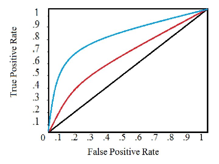
ROC curve In the case of certain classification algorithms, the classifier may depend on a parameter. Different values of the parameter will give different classifiers and these in turn give different values to TPR and FPR. The ROC curve is the curve obtained by plotting in the ROC space the points (TPR , FPR) obtained by assigning all possible values to the parameter in the classifier

ROC curve The closer the ROC curve is to the top left corner (0, 1) of the ROC space, the better the accuracy of the classifier. Among the three classifiers A, B, C with ROC curves , the classifier C is closest to the top left corner of the ROC space. Hence, among the three, it gives the best accuracy in predictions.

The body mass index (BMI) of a person is defined as (weight(kg)/height(m)2 ). Researchers have established a link between BMI and the risk of breast cancer among women. The higher the BMI the higher the risk of developing breast cancer. The critical threshold value of BMI may depend on several parameters like food habits, socio-cultural-economic background, life-style, etc Gives real data of a breast cancer study with a sample having 100 patients and 200 normal persons. The table also shows the values of TPR and FPR for various cut-off values of BMI.

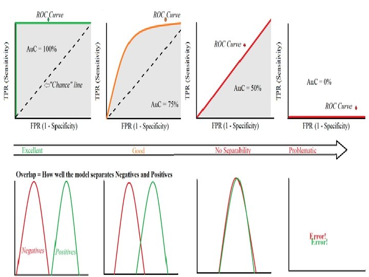
Area under the ROC curve (AUC) The measure of the area under the ROC curve is denoted by the acronym AUC. The value of AUC is a measure of the performance of a classifier. For the perfect classifier, AUC = 1. 0.

Bayesian classifier and ML estimation The Bayesian classifier is an algorithm for classifying multiclass datasets. This is based on the Bayes’ theorem in probability theory. Bayes in whose name theorem is known was an English statistician who was known for having formulated a specific case of a theorem that bears his name. The classifier is also known as “naive Bayes Algorithm” where the word “naive” is an English word with the following meanings: simple,

Bayesian probability Notion of probability talks about partial beliefs Bayesian estimation calculates the validity of a proposition based on � Prior estimate � New relevant evidence

Conditional probability The probability of the occurrence of an event A given that an event B has already occurred is called the conditional probability of A given B and is denoted by P(A∣B)= P(A∩B)/ P(B) if P(B) ≠ 0:

Independent events Two events A and B are said to be independent if P(A∩B)= P(A)P(B) Three events A; B; C are said to be pair-wise independent if P(B ∩C)= P(B)P(C) P(C ∩A)= P(C)P(A) P(A∩B)= P(A)P(B) Three events A; B; C are said to be mutually independent if P(B ∩C)= P(B)P(C) P(C ∩A)= P(C)P(A) P(A∩B)= P(A)P(B) P(A∩B ∩C)= P(A)P(B)P(C) In general, a family of k events A 1; A 2; : : : ; Ak is said to be mutually independent if for any subfamily consisting of Ai 1; : : : Aim we have P(Ai 1 ∩: : : ∩Aim)= P(Ai 1): : : P(Aim):

Bayes’ theorem Let A and B any two events in a random experiment. If P(A)≠ 0, then P(B∣A)= P(A∣B)P(B) / P(A) The importance of the result is that it helps us to “invert” conditional probabilities, that is, to express the conditional probability P(A∣B) in terms of the conditional probability P(B∣A).

Bayes Theorem How to find the probability of a hypothesis given the data P(h/D) used to find most probable hypothesis P(h/D) = [P(D/h) P(h)]/P(D) Law of products states that P(h. D) = P(h) P(D/h) P(Dh)= P(D) P(h/D) Commutative P(h) P(D/h) = P(D) P(h/D)

Bayes’ theorem The following terminology is used in this context: A is called the proposition and B is called the evidence. � P(A) is called the prior probability of proposition and P(B) is called the prior probability of evidence � P(A∣B) is called the posterior probability of A given B. � P(B∣A) is called the likelihood of B given A. �

Generalisation Let the sample space be divided into disjoint events B 1; B 2; : : : ; Bn and A be any event. P(Bk∣A)= P(A∣B k)P(Bk) / n P(A∣B )P(B ) ∑ i=1 i i

Problem 1 Consider a set of patients coming for treatment in a certain clinic. Let A denote the event that a “Patient has liver disease” and B the event that a “Patient is an alcoholic. ” It is known from experience that 10% of the patients entering the clinic have liver disease and 5% of the patients are alcoholics. Also, among those patients diagnosed with liver disease, 7% are alcoholics. Given that a patient is alcoholic, what is the

Problem 1 Using the notations of probability, P(A)= 10% = 0. 10 P(B)= 5% = 0. 05 P(B∣A)= 7% = 0. 07 P(A∣B)= P(B∣A)P(A) / P(B) = 0. 07× 0. 10/ 0. 05 = 0. 14

Problem 2 Three factories A, B, C of an electric bulb manufacturing company produce respectively 35%, 35% and 30% of the total output. Approximately 1. 5%, 1% and 2% of the bulbs produced by these factories are known to be defective. If a randomly selected bulb manufactured by the company was found to be defective, what is the probability that the bulb was manufactures in factory A?

Problem 2 Let A; B; C denote the events that a randomly selected bulb was manufactured in factory A, B, C respectively. Let D denote the event that a bulb is defective. We have the following data: P(A)= 0. 35; P(B)= 0. 35; P(C)= 0. 30 P(D∣A)= 0. 015; P(D∣B)= 0. 010; P(D∣C)= 0. 020 We are required to find P(A∣D). By the generalisation of the Bayes’ theorem we have: P(A∣D)= P(D∣A)P(A)/[ P(D∣A)P(A)+P(D∣B)P(B)+P(D∣C)P(C) ] =0. 015× 0. 35/015× 0. 35+0. 010× 0. 35+0. 020× 0. 30 = 0. 356

Problem 3 A patient has cancer or not A patient takes a lab test and result comes back positive. The test returns a correct positive result in only 98% of the cases in which the disease actually present, and a correct negative result is only 97% of the cases in which the disease is not present. Furthermore. 008 of the entire population have this cancer

Problem 3 P(cancer) P(+/ cancer) P(cancer/+) P( cancer/+) P(-/cancer) P(-/ cancer)

Naive Bayes algorithm. Assumption The naive Bayes algorithm is based on the following assumptions: All the features are independent and are unrelated to each other. Presence or absence of a feature does not influence the presence or absence of any other feature. � The data has class-conditional independence, which means that events are independent so long as they are conditioned on the same class value. � These assumptions are, in general, true in many real world problems. It is because of these assumptions, the algorithm is called a naive �

Naive Bayes algorithm Suppose we have a training data set consisting of N examples having n features. Let the features be named as (F 1; : : : ; Fn). A feature vector is of the form (f 1; f 2; : : : ; fn). Associated with each example, there is a certain class label. Let the set of class labels be {c 1; c 2; : : : ; cp}.

Naive Bayes algorithm Suppose we are given a test instance having the feature vector X =(x 1; x 2; : : : ; x n): We are required to determine the most appropriate class label that should be assigned to the test instance. For this purpose we compute the following conditional probabilities P(c 1∣X); P(c 2∣X); : : : ; P(c p ∣X): and choose the maximum among them.

Naive Bayes algorithm Let the maximum probability be P(ci∣X). Then, we choose ci as the most appropriate class label for the training instance having X as the feature vector. The direct computation of the probabilities given are difficult for a number of reasons. The Bayes’ theorem can b applied to obtain a simpler method.

Computation of probabilities P(ck ∣X)= P(X∣ck)P(ck)/ P(X) Since, by assumption, the data has classconditional independence, we note that the events “x 1∣ck”, “x 2∣ck”, ⋯, xn∣ck are independent P(X∣ck)= P((x 1; x 2; : : : ; xn)∣ck) = P(x 1∣ck)P(x 2∣ck)⋯P(xn∣ck) P(ck∣X)= P(x 1∣ck)P(x 2∣ck)⋯P(xn∣ck)P(ck)/ P(X) : Since the denominator P(X) is independent of the class labels, we have P(ck∣X)∝ P(x 1∣ck)P(x 2∣ck)⋯P(xn∣ck)P(ck): So it is enough to find the maximum among the

Computation of probabilities The various probabilities in the above expression are computed as follows: P(ck)= No. of examples with class label ck/ Total number of examples P(xj ∣ck)= No. of examples with jth feature equal to x j and class label ck/ No. of examples with class label ck

The Naive Bayes Algorithm: Let there be a training data set having n features (F 1; : : : ; Fn). Let f 1 denote an arbitrary value of F 1 , f 2 of F 2, and so on. (f 1; f 2; : : : ; fn). Let the set of class labels be {c 1; c 2; : : : ; cp}. Let there be given a test instance having the feature vector X =(x 1; x 2; : : : ; x n): We are required to determine the most appropriate class label that should be assigned to the test instance.

The Naive Bayes Algorithm: Step 1. Compute the probabilities P(ck) for k = 1; : : : ; p. Step 2. Form a table showing the conditional probabilities P(f 1∣ck); P(f 2∣ck); : : : ; P(fn ∣ck) for all values of f 1; f 2; : : : ; fn and for k = 1; : : : ; p. Step 3. Compute the products � qk = P(x 1∣ck)P(x 2∣ck)⋯P(xn ∣c k)P(ck) � for k = 1; : : : ; p. Step 4. Find j such qj = max{q 1; q 2; : : : ; q p}. Step 5. Assign the class label cj to the test instance X.

Problem Consider a training data set consisting of the fauna of the world. Each unit has three features named “Swim”, “Fly” and “Crawl”. Let the possible values of these features be as follows: Swim Fast, Slow, No Fly Long, Short, Rarely, No Crawl Yes, No For simplicity, each unit is classified as “Animal”, “Bird” or “Fish”. Use naive Bayes algorithm to classify a particular species if its features are (Slow, Rarely, No)?

Sl. No. Swim Fly Crawl Class 1 Fast No No Fish 2 Fast No Yes Animal Slow No No Animal 4 Fast No No Animal 5 No Short No Bird 6 No Short No Bird 7 No Rarely No Animal 8 Slow No Yes Animal 9 Slow No No Fish 10 Slow No Yes Fish 11 No Long No Bird 12 Fast No No Bird 3

The features are F 1 = “Swim”; F 2 = “Fly”; F 3 = “Crawl”: The class labels are c 1 = “Animal”; c 2 = “ Bird”; c 3 = “Fish”: The test instance is (Slow, Rarely, No) and so we have: x 1 = “Slow”; x 2 = “Rarely”; x 3 = “No”:

P(c 1)= No. of records with class label “Animal” Total number of examples = 5/12 P(c 2)= No. of records with class label “Bird” Total number of examples = 4/12 P(c 3)= No of records with class label “Fish” Total number of examples = 3/12

Condition Probabilities

Using numeric features with naive Bayes algorithm The naive Bayes algorithm can be applied to a data set only if the features are categorical. This is so because, the various probabilities are computed using the various frequencies and the frequencies can be counted only if each feature has a limited set of values. If a feature is numeric, it has to be discretized before applying the algorithm. The discretization is effected by putting the numeric values into categories known as bins. Becauseofthis discretization is also known as binning. This is ideal when there are large amounts of data.

Using numeric features with naive Bayes algorithm There are several different ways to discretize a numeric feature. 1. If there are natural categories or cut points in the distribution of values, use these cut points to create the bins. For example, let the data consists of records of times when certain activities were carried out. 2. If there are no obvious cut points, we may discretize the feature using quantiles. We may divide the data into three bins with tertiles, four bins with quartiles, or five bins with quintiles, etc

Short answer questions What is cross-validation in machine learning? What is meant by 5 × 2 cross-validation? What is meant by leave-one-out cross validation? What is meant by the confusion matrix of a binary classification problem. Define the following terms: precision, recall, sensitivity, specificity. What is ROC curve in machine learning? What are true positive rates and false positive rates in machine learning? What is AUC in relation to ROC curves?

Short answer questions What are the assumptions under the naive Bayes algorithm? Why is naive Bayes algorithm “naive”? Given an instance X of a feature vector and a class label ck, explain how Bayes theorem is used to compute the probability P(ck ∣X). What does a naive Bayes classifier do? What is naive Bayes used for? Is naive Bayes supervised or unsupervised? Why? What is meant by the likelihood of a random sample taken from population? How do we use numeric features in naive Bayes algorithm?

Long answer questions Explain cross-validation in machine learning. Explain the different types of cross-validations. What is meant by true positives etc. ? What is meant by confusion matrix of a binary classification problem? Explain how this can be extended to multi-class problems. What are ROC space and ROC curve in machine learning? In ROC space, which points correspond to perfect prediction, always positive prediction and always negative prediction? Why? Consider a two-classification problem of predicting whether a photograph contains a man or a woman. Suppose we have a test dataset of 10 records with expected outcomes and a set of predictions from

Long answer questions (a) (b) Expected Predicted 1 man woman 2 man 3 woman 4 man 5 woman 6 woman 7 woman 8 man 9 man woman 10 woman Compute the confusion matrix for the data. Compute the accuracy, precision, recall, sensitivity and specificity of the data.

Long answer questions Suppose 10000 patients get tested for flu; out of them, 9000 are actually healthy and 1000 are actually sick. For the sick people, a test was positive for 620 and negative for 380. For the healthy people, the same test was positive for 180 and negative for 8820. Construct a confusion matrix for the data and compute the accuracy, precision and recall for the data.

Long answer questions Given the following data, construct the ROC curve of the data. Compute the AUC. Threshold TP TN FP FN 1 0 25 0 29 2 7 25 0 22 3 18 24 1 11 4 26 20 5 3 5 29 11 14 0 6 29 0 25 0 7 29 0 25 0

Long answer questions Given the following hypothetical data at various cut-off points of mid-arm circumference to detect low birthweight construct the ROC curve for the data.

Long answer questions Mid-arm circumference weight (cm) ≤ 8. 3 ≤ 8. 4 ≤ 8. 5 ≤ 8. 6 ≤ 8. 7 ≤ 8. 8 ≤ 8. 9 ≤ 9. 0 ≤ 9. 1 ≤ 9. 2 and above Normal birth-weight TP 13 24 73 90 113 119 121 125 127 130 Low birth. TN 867 844 826 800 783 735 626 505 435 0

Long answer questions State Bayes theorem and illustrate it with an example. Explain naive Bayes algorithm. Explain the general MLE method for estimating the parameters of a probability distribution. Find the ML estimate for the parameter p in the binomial distribution whose probability function is f(x)=(n x )px(1−p)n−x; x = 0; 1; 2; : : : ; n Compute the ML estimate for the parameter in the Poisson distribution whose probability function is f(x)= e− x x! ; x = 0; 1; 2; : : : Find the ML estimate of the parameter p in the geometric distribution defined by the probability mass function f(x)=(1−p)px; x = 1; 2; 3; : : :

Use naive Bayes algorithm to determine whether a red domestic SUV car is a stolen car or not using the following data:

Based on the following data determine the gender of a person having height 6 ft. , weight 130 lbs. and foot size 8 in. (use naive Bayes algorithm).

Given the following data on a certain set of patients seen by a doctor, can the doctor conclude that a person having chills, fever, mild headache and without running nose has the flu?