Module 3 linear regression Wei Metropolitan State University

Module 3 linear regression Wei Metropolitan State University Saint Paul, MN USA

Learning objectives and outcomes • Know how to fit a linear regression model to data in SPSS • Know how to estimate (in SPSS) and interpret the slope and intercept of a linear regression model • Know how to test whethere is a significant relationship between two variables • Know how to do a residual analysis

When to use regression analysis • ANOVA: – The independent variable(s) is Categorical • gender, type of group, temperature levels – The dependent variable is numeric • Regression (linear and multiple regression) – The independent variable (s) is numeric • age, weight, concentration, etc. – The dependent variable is also numeric

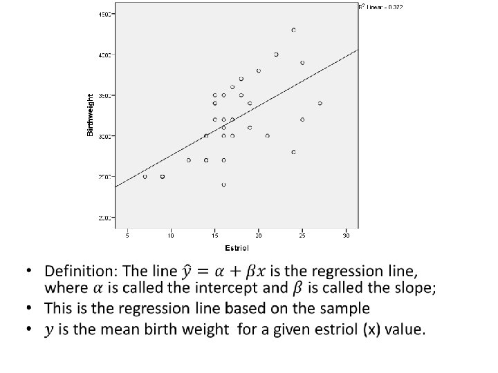
Regression line Case study: Obstetricians sometimes order tests to measure estriol levels (雌激素三醇水平) from 24 -hour urine specimens taken from pregnant women who are near term because level of estriol has been found to be related to infant birthweight. The test can provide indirect evidence of an abnormally small fetus. The data from a sample of 31 pregnant women and their babies’ birth weight (measured as g) was provided by the Greene-Touchstone study in 1963. The data is online. Do a scatter plot to see the relationship between estriol level and birth weight. • Graphs->Legacy dialogs->Simple scatter plot->choose your x and y • Double click the graph to activate it->Add fit line to total

Types of relationship • 25 20 y 15 10 5 0 0 2 4 6 x 8 10 12

Types of relationship y • 20 18 16 14 12 10 8 6 4 2 0 0 5 x 10 15

Types of relationship • 3, 5 3 2, 5 y 2 1, 5 1 0, 5 0 0 2 4 6 x 8 10 12

Least square regression line •

How to obtain least square regression line •

How to obtain least square regression Example: A student wonders if tall women tend to date taller men than do short women. She measures herself, her dormitory roommates and the women in the adjoining rooms. Then she measures the height of man that each woman dates, in inches. Is there a significant correlation between the heights of women and the heights of men they date? Is there anything about the data that might make the results questionable? Women 66 64 (167 cm) Men 69 68 (175 cm) 68 65 70 68 70 (178 cm) 71 (180 cm)

How to obtain least square regression •

Use SPSS to get the regression model • Analyze->Regression->Linear->choose your dependent and independent variables

Least regression line using SPSS •

Interpret the parameters •

Activity 1 The data in the following table give the infantmortality rates per 1000 livebirths in the U. S. for the period 1960 -2005. • Generate a scatter plot and fit a regression line relating infant-mortality rate to chronological year using the data. What is the equation of the regression line?

Activity 1 • If the present trends continue, what would be the predicted infant-mortality rate in 2010? • In which year (round up to the nearest integer), the infant-mortality rate will be down to 4. 0 per 1000 livebirths? a) 930. 095, 0. 462 b) 1. 475, 2005 c) 0. 462, 930. 095 d) 906. 995, 2004

Activity 1 • Interpret the slope in the context – When the birth rate increases by 1, the death rate decreases by 0. 462 per 1000 birth

Test of slope •

Test of slope •

Test of slope •

ANOVA test of slope • Residual component Regression component

Test of slope and confidence interval of slope and intercept • You can either do an ANOVA or a T-test on the slope. • ANOVA and T-test conclusions are consistent • Analyze -> Regression-> Linear-> Choose your dependent and independent variables • SPSS can also generate the confidence interval estimation for slope and intercept • SPSS can also produce the standard error of slope and intercept • Check “confidence intervals” in statistics

Four steps of hypothesis testing •

Example 2 •

Example 2 output

Example 2 output The confidence interval for the slope is (53. 863, 145. 216) There is a significant linear relationship between the x and y

Activity 2 • Continue with activity 1, assess whether the relationship between year and infantmortality rate is significant

Activity 2 • What is the 95% confidence interval of the slope? What can you conclude based on the 95% confidence interval? • Do you think the trend will continue to indefinitely? Why?

Does your line fit the data well? •

Residual analysis • Residual plot: x: predicted value (y); y: residuals • In SPSS, in the option of “plot”, choose “ZPRED” as the x value and choose “ZRESID” as the y. • Assumptions to run regression analysis – Linearity assumption – Equal variance assumption – Normality assumption (true if sample size is large) – Independence ( usually violated in time series data) • Outliers and influential points – Influential points: Defined as the outliers on the xdirection

Linearity assumption Linear Not Linear

Assumption is violated Equal variance assumption Assumption is violated Assumption is satisfied

Outlier and influential points • Definition: an outlier is a point lying far away from the other data points • Definition: an influential point is a point strongly affecting the graph of the regression line 4 3, 5 3 Without outlier 2, 5 2 With outlier 1, 5 1 0, 5 0 0 0, 5 1 1, 5 2 2, 5 3 3, 5 4 4, 5

Example 3 • One outlier

Example • Linearity assumption is reasonable • Equal variance is violated: higher estriol levels have more variability

Activity 3 •

Variance stabling transformation • Square root transformation of the dependent variable • Ln transformation of the dependent variable • Re-do the residual plot to check the equal variance assumption