Module 2 Revealing of tracking signals and radar

Module 2. Revealing of tracking signals and radar surveillance Topic 2. 1 THEORY OF TRACKING SIGNALS REVEALING Lecture 2. 1. 1 SIGNALS AND HINDRANCES CHARACTERISTICS

Radar signal characteristics A radar system uses a radio frequency electromagnetic signal reflected from a target to determine information about that target. In any radar system, the signal transmitted and received will exhibit many of the characteristics described below.

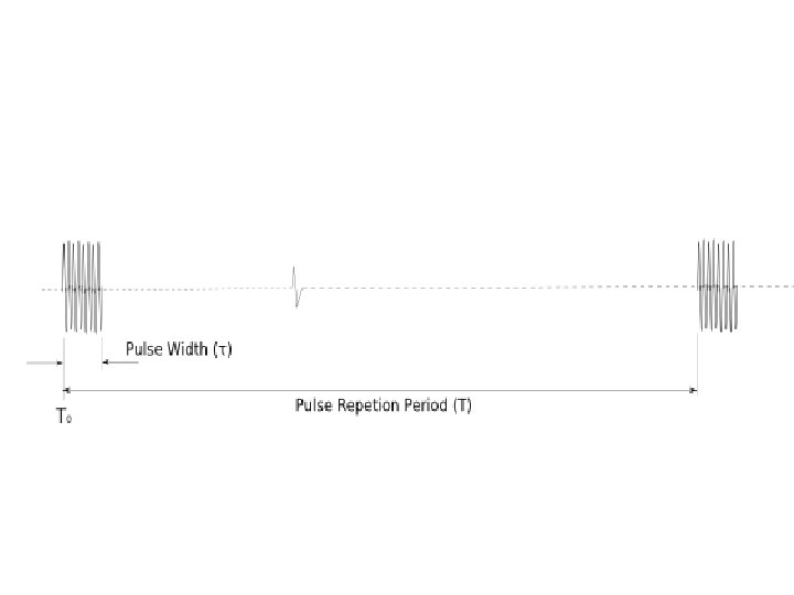
The radar signal in the time domain The diagram below shows the characteristics of the transmitted signal in the time domain. Note that the x axis is exaggerated to make the explanation clearer.

Carrier The carrier is an RF signal, typically of microwave frequencies, which is usually (but not always) modulated to allow the system to capture the required data. In simple ranging radars, the carrier will be pulse modulated and in continuous wave systems, such as Doppler radar, modulation may not be required. Most systems use pulse modulation, with or without other supplementary modulating signals. Note that with pulse modulation, the carrier is simply switched on and off in sync with the pulses; the modulating waveform does not actually exist in the transmitted signal and the envelope of the pulse waveform is extracted from the demodulated carrier in the receiver. Although obvious when described, this point is often missed when pulse transmissions are first studied, leading to misunderstandings about the nature of the signal.

Pulse width The pulse width ( ) of the transmitted signal determines the dead zone. While the radar transmitter is active, the receiver input is blanked to avoid the amplifiers being swamped (saturated) or, (more likely), damaged. A simple calculation reveals that a radar echo will take approximately 10. 8 μs to return from a target 1 standard mile away (counting from the leading edge of the transmitter pulse (T 0), (sometimes known as transmitter main bang)). For convenience, these figures may also be expressed as 1 nautical mile in 12. 4 μs or 1 kilometre in 6. 7 μs. (For simplicity, all further discussion will use metric figures. ) If the radar pulse width is 1 μs, then there can be no detection of targets closer than about 150 m, because the receiver is blanked.

Pulse repetition frequency (PRF) In order to build up a discernible echo, most radar systems emit pulses continuously and the repetition rate of these pulses is determined by the role of the system. An echo from a target will therefore be 'painted' on the display or integrated within the signal processor every time a new pulse is transmitted, reinforcing the return and making detection easier. The higher the PRF that is used, then the more the target is painted. However with the higher PRF the range that the radar can "see" is reduced. Radar designers try to use the highest PRF possible commensurate with the other factors that constrain it, as described below.

Staggered PRF is where the time between interrogations from radar changes slightly. The change of repetition frequency allows the radar, on a pulse-topulse basis, to differentiate between returns from itself and returns from other radar systems with the same frequency. Without stagger any returns from another radar on the same frequency would appear stable in time and could be mistaken for the radar's own returns. With stagger the radar’s own targets appear stable in time in relation to the transmit pulse, whilst the 'jamming' echoes are moving around in time (uncorrelated), causing them to be rejected by the receiver.

Clutter (also termed ground clutter) is a form of radar signal contamination. It occurs when fixed objects close to the transmitter—such as buildings, trees, or terrain (hills, ocean swells and waves)—obstruct a radar beam and produce echoes. The echoes resulting from ground clutter may be large in both areal size and intensity. The effects of ground clutter fall off as range increases usually due to the curvature of the earth and the tilt of the antenna above the horizon. Without special processing techniques, targets can be lost in returns from terrain on land or waves at sea.

Sensitivity time control (STC) STC is used to avoid saturation of the receiver from close in ground clutter by adjusting the attenuation of the receiver as a function of distance. More attenuation is applied to returns close in and is reduced as the range increases.

Unambiguous range Single PRF

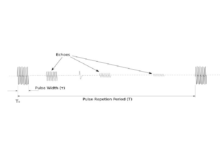
In simple systems, echoes from targets must be detected and processed before the next transmitter pulse is generated if range ambiguity is to be avoided. Range ambiguity occurs when the time taken for an echo to return from a target is greater than the pulse repetition period (T). These 'second echoes' would appear on the display to be targets closer than they really are.

Consider the following example : if the radar antenna is located at around 15 m above sea level, then the distance to the horizon is pretty close, (perhaps 15 km). Ground targets further than this range cannot be detected, so the PRF can be quite high; a radar with a PRF of 7. 5 k. Hz will return ambiguous echoes from targets at about 20 km, or over the horizon. If however, the PRF was doubled to 15 k. Hz, then the ambiguous range is reduced to 10 km and targets beyond this range would only appear on the display after the transmitter has emitted another pulse. A target at 12 km would appear to be 2 km away, although the strength of the echo would be much lower than that from a genuine target at 2 km.

The maximum non ambiguous range varies inversely with PRF and is given by: If a longer range is required with this simple system, then lower PRFs are required and it was quite common for early search radars to have PRFs as low as 1 k. Hz, giving an unambiguous range out to 150 km. However, lower PRFs mean other problems, including poorer target painting and velocity ambiguity in Pulse-Doppler systems

Multiple PRF Modern radars frequently use PRFs in the hundreds of kilohertz and stagger the interval between pulses to allow the correct range to be determined. With a staggered PRF, a 'packet' of pulses is transmitted, each pulse a slightly different interval after the last (or viewed a different way; delayed variable amounts from the reference trigger). At the end of the packet, the timing returns to its original value, in sync with the trigger.

This means that the second and subsequent echoes will appear in the receiver's processing circuits at slightly different times, relative to the current transmitter pulse. These echoes can then be correlated with their associated T 0 pulse in the packet to build up a true range value. Echoes from other T 0 triggers, eg 'ghost echoes', will therefore recede from the display or be canceled in the signal processor, leaving only the true echoes which can then be used to calculate range.

MUR (Maximum Unambiguous Range) for a Pulsed Stagger radar is calculated using the TSP (Total Sequence Period). TSP is defined as the total time it takes for the Pulsed pattern to repeat. This can be found by the addition of all the elements in the stagger sequence. The formula is: where C is the speed of light and TSP is the addition of all the positions of the stagger sequence usually in microseconds.

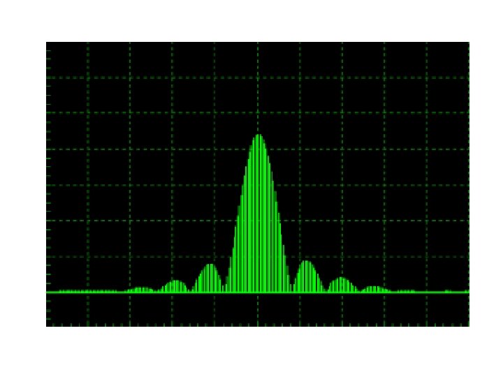
The radar signal in the frequency domain Pure CW radars appear as a single line on a Spectrum analyser display and when modulated with other sinusoidal signals, the spectrum differs little from that obtained with standard analogue modulation schemes used in communications systems, such as Frequency Modulationand consist of the carrier plus a relatively small number of sidebands. When the radar signal is modulated with a pulse train as shown above, the spectrum becomes much more complicated and far more difficult to visualise.

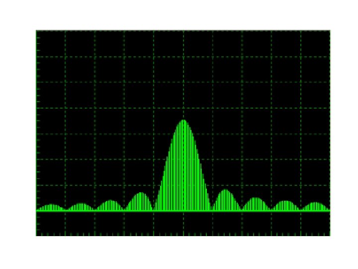
Basic Fourier analysis shows that any repetitive complex signal consists of a number of harmonically related sine waves. The radar pulse train is a form of square wave, the pure form of which consists of the fundamental plus all of the odd harmonics. The exact composition of the pulse train will depend on the pulse width and PRF, but mathematical analysis can be used to calculate all of the frequencies in the spectrum. When the pulse train is used to modulate a radar carrier, the typical spectrum shown on the left will be obtained.

Examination of this spectral response shows that it contains two basic structures. The Coarse Structure; (the peaks or 'lobes' in the diagram on the left) and the Fine Structure which contains the individual frequency components as shown below. The Envelope of the lobes in the Coarse Structure is given by: . Note that the pulse width ( ) appears on the bottom of this equation and determines the lobe spacing. Smaller pulse widths result in wider lobes and therefore greater bandwidth.

Examination of the spectral response in finer detail, as shown on the right, shows that the Fine Structure contains individual lines or spot frequencies. The formula for the fine structure is given by and since the period of the PRF (T) appears at the top of the fine spectrum equation, there will be fewer lines if higher PRFs are used. These facts affect the decisions made by radar designers when considering the tradeoffs that need to be made when trying to overcome the ambiguities that affect radar signals.

Pulse profiling If the rise and fall times of the modulation pulses are zero, (e. g. the pulse edges are infinitely sharp), then the sidebands will be as shown in the spectral diagrams above. The bandwidth consumed by this transmission can be huge and the total power transmitted is distributed over many hundreds of spectral lines. This is a potential source of interference with any other device and frequency-dependent imperfections in the transmit chain mean that some of this power never arrives at the antenna. In reality of course, it is impossible to achieve such sharp edges, so in practical systems the sidebands contain far fewer lines than a perfect system. If the bandwidth can be limited to include relatively few sidebands, by rolling off the pulse edges intentionally, an efficient system can be realised with the minimum of potential for interference with nearby equipment.

However, the trade-off of this is that slow edges make range resolution poor. Early radars limited the bandwidth through filtration in the transmit chain, e. g. the waveguide, scanner etc, but performance could be sporadic with unwanted signals breaking through at remote frequencies and the edges of the recovered pulse being indeterminate. Further examination of the basic Radar Spectrum shown above shows that the information in the various lobes of the Coarse Spectrum is identical to that contained in the main lobe, so limiting the transmit and receive bandwidth to that extent provides significant benefits in terms of efficiency and noise reduction.

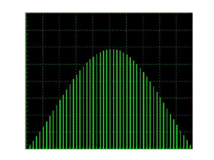
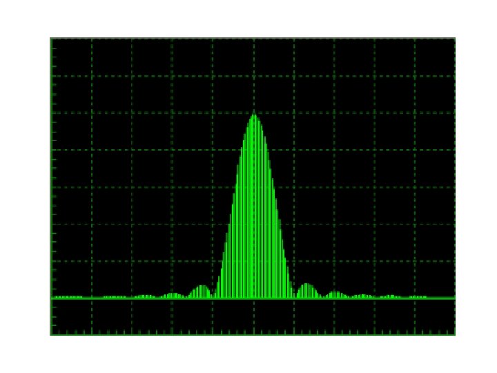
Recent advances in signal processing techniques have made the use of pulse profiling or shaping more common. By shaping the pulse envelope before it is applied to the transmitting device, say to a cosine law or a trapezoid, the bandwidth can be limited at source, with less reliance on filtering. When this technique is combined with pulse compression, then a good compromise between efficiency, performance and range resolution can be realized. The diagram shows the effect on the spectrum if a trapezoid pulse profile is adopted. It can be seen that the energy in the sidebands is significantly reduced compared to the main lobe and the amplitude of the main lobe is increased.

Similarly, the use of a cosine pulse profile has an even more marked effect, with the amplitude of the sidelobes practically becoming negligible. The main lobe is again increased in amplitude and the sidelobes correspondingly reduced, giving a significant improvement in performance. There are many other profiles that can be adopted to optimise the performance of the system, but cosine and trapezoid profiles generally provide a good compromise between efficiency and resolution and so tend to be used most frequently.

Unambiguous velocity

This is an issue only with a particular type of system; the Pulse-Doppler radar, which uses the Doppler effect to resolve velocity from the apparent change in frequency caused by targets that have net radial velocities compared to the radar device. Examination of the spectrum generated by a pulsed transmitter, shown above, reveals that each of the sidebands, (both coarse and fine), will be subject to the Doppler effect, another good reason to limit bandwidth and spectral complexity by pulse profiling.

Consider the positive shift caused by the closing target in the diagram which has been highly simplified for clarity. It can be seen that as the relative velocity increases, a point will be reached where the spectral lines that constitute the echoes are hidden or aliased by the next sideband of the modulated carrier. Transmission of multiple pulse-packets with different PRF-values, eg staggered PRFs, will resolve this ambiguity, since each new PRF value will result in a new sideband position, revealing the velocity to the receiver.

The maximum unambiguous target velocity is given by:

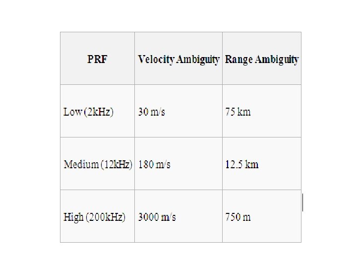
Typical system parameters Taking all of the above characteristics into account means that certain constraints are placed on the radar designer. For example, a system with a 3 GHz carrier frequency and a pulse width of 1 us will have a carrier period of approximately 333 ps. Each transmitted pulse will contain about 3000 carrier cycles and the velocity and range ambiguity values for such a system would be:

RADAR SIGNALS REVEALING AGAINST HINDRANCES AS THE STATISTICAL PROBLEM Reflected signal has useful information. However at receiver input together with a useful signal hindrances operate also mutual hindrances, internal receiver noise. So decision about target presence or absence cannot be completely reliable. Decision is made with some probability of errors. `

For solving problems of detection it is necessary to have apriori (i. e. previous to experience, in this case - before detection) data about structure of useful signal and hindrances. Such data (signal form, statistical characteristics of a hindrance, polarization differences between signal and hindrance etc. ) always are available.

They allow finding optimal methods of signals processing. It gives possibility to create device for optimal signal processing. At radar detection it is necessary to make decision about target presence or absence and for this it is necessary to check up two mutually exclusive hypotheses: H 1 - target is present and H 0 target is not present. Operator can make one of two decisions: А 1 - target is present and А 0 - target is not present.

This leads to the following four situations: 1. Decision А 1 is made under a condition when hypotheses H 1 is true. This situation we will designate А 1 H 1 and name correct detection; 2. Decision А 0 is made under a condition when hypotheses H 1 is true. This situation we will designate А 0 H 1 and name target miss; 3. Decision А 1 is made under a condition when hypotheses H 0 is true. This situation we will designate А 1 H 0 and name false alarm; 4. Decision А 0 is made under a condition when hypotheses H 0 is true. This situation we will designate А 0 H 0 and name correct non detection.

Occurrence of any from four situations is random event, for the quantitative description of which conditional probabilities are introduced: - Probability of correct detection D = p (А 1/H 1); - Probability of false alarm F = p (А 1/H 0); - Probability of target miss D 0 = p (A 0/H 1); - Probability of correct non detection F 0 = p (A 0/H 0).

According to definition following equalities are valid: D + D 0 = 1, F + F 0 = 1, testifying that from four introduced values only two are independent. In a radar-location it is accepted to use probability of correct detection D and probability of false alarm F.

On the one hand for radar it is expedient to increase probability of correct detection D but then the probability of false alarm F will increase. I. e. the compromise is necessary for the choice of D and F.

However use of two indicators not always is convenient. Therefore generalized error (average risk) is introduced : ř = r 01 p (A 0 H 1) + r 10 p (A 1 H 0). Radar is better when it provides smaller value of average risk ř.

After transformations: ř = r 01 p (H 1) [1 - (D - l 0 F)]. From here we can see that ř is less when difference I = (D - l 0 F) bigger. So, proceeding from minimization requirements for ř, the best will be that radar which provides bigger value of I, optimum radar - for which value of I is maximum. As rule, the value of D try to provide not less than 0, 85, and F = 10 -6. . . 10 -8. For ATC radars usually: D = 0. 9, and F = 10 -7.

Likelihood ratio Probability of correct detection D can be determined by integration of ω1 (y) - probability density distribution for the sum of useful and parasitic signals: ∞ D = ∫ ω1 (y) dy. Y 0

Probability of false alarm - by integration of ω0 (y) - probability density distribution of parasitic signal: ∞ F = ∫ ω0 (y) dy. Y 0

Hence, it is possible to receive relative criteria - the ratio of probability densities: l = ω1 (y) / ω0 (y), which is called likelihood ratio (соотношение правдоподобия).

When designing radar it is necessary to increase likelihood ratio, which essentially depends on a kind of detected signals, degree of its parameters knowledge, and also from statistic characteristics of noise and hindrance. It means, that to everyone type of detected signal corresponds its own receiver.

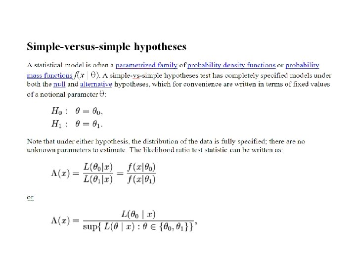
Likelihood-ratio test In statistics, a likelihood ratio test is used to compare the fit of two models one of which is nested within the other. Both models are fitted to the data and their log-likelihood recorded. The test statistic (usually denoted D) is twice the difference in these log-likelihoods:

The model with more parameters will always fit at least as well (have a greater log-likelihood). Whether it fits significantly better and should thus be preferred can be determined by deriving the probability or p-value of the obtained difference D.

In many cases, the probability distribution of the test statistic can be approximated by a chi-square distribution with (df 1 − df 2) degrees of freedom, where df 1 and df 2 are the degrees of freedom of models 1 and 2 respectively. The test requires nested models, that is, models in which the more complex one can be transformed into the simpler model by imposing a set of linear constraints on the parameters.

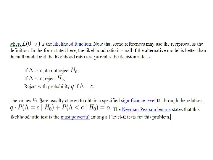
Background The likelihood ratio, often denoted by Λ (the capital Greek letter lambda), is the ratio of the likelihood function varying the parameters over two different sets in the numerator and denominator. A likelihood-ratio test is a statistical test for making a decision between two hypotheses based on the value of this ratio.

END.