Module 2 FUNDAMENTAL CONCEPTS BASIC STATISTICS 1 2

Module 2 FUNDAMENTAL CONCEPTS (BASIC STATISTICS) 1

2. 1 THE DISTINCTION BETWEEN POPULATION AND SAMPLE Population : Entire group of individuals that we want information about. In the context of environmental statistics “individuals” can be marine organisms, concentration of air pollutants at different times of the day or locations, people, birds, elephants and trees. Sample : Part of the population that we actually examine in order to gather information about the population. By definition, is a subset of a population. 2

ILLUSTRATION M 2. 1 In a chemical process plant, there is a large shed that is used to store drums of scheduled wastes waiting to be collected by the scheduled waste transportation contractor. A requirement of the Environmental Quality (Scheduled Waste) Regulation, 2005 is that all drums should be labelled with the correct scheduled waste code. A DOE enforcement officer come to the process plant to inspect whether the plant comply with the requirements of the regulation by taking samples of the waste in the drums and sent to the laboratory for analysis. It is estimated that there are 500 drums at the time of the inspection. 3

ILLUSTRATION M 2. 1 Does the DOE officer has to take samples from every drum? What problems can arise if samples from every drum have to be taken? What would be the implications to select a number of drums only to represent the total number within the storage shed? What constitute the “population” and the “sample” for this case? 4

ILLUSTRATION M 2. 2 In the marine ecosystem, the targeted marine organisms that we want to sample are usually in the form of different groups of marine organism population. The mesh size of the plankton net generally determines the section in the population that we get in the sample. If we use a 300 m mesh size, we are going to catch only zooplankton sample from zooplankton population in the areas. However if we decide to use 150 m mesh size plankton net, we are going to sample both of the phyto-plankton and zooplankton net from both phyto- and zoo-plankton populations. What is the relevant population when we decide to use the 150 m mesh size plankton net for sampling? 5

ILLUSTRATION M 2. 2 We also conduct randomized sampling on the inter-tidal mudflat in environmental studies. Typically, we have to choose a representative stretch of exposed mudflat perpendicular or parallel to the high water marks. Line Transect is then laid down and quadrate of certain sizes (m 2) can be randomly thrown on both sides along the transect line. Samples of the marine organism can now be taken whether on the surface or in the sediment populations within the quadrates. What is the population of interest from which the samples were to be taken? What about the sampled population? 6

2. 2 STATISTICAL DISTRIBUTION In statistics, a distribution is the set of all possible values for terms that represent defined events. The value of a term, when expressed as a variable, is called a random variable. Two major types of statistical distributions. discrete random variable. continuous random variable. 7

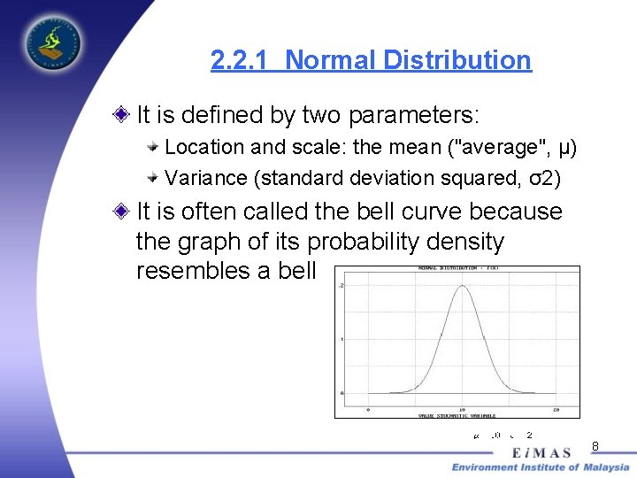
2. 2. 1 Normal Distribution It is defined by two parameters: Location and scale: the mean ("average", μ) Variance (standard deviation squared, σ2) It is often called the bell curve because the graph of its probability density resembles a bell 8

2. 2. 1 Normal Distribution The standard normal distribution is the normal distribution with a mean of zero and a variance of one. The use of the normal model can be theoretically justified by assuming that many small, independent effects are additively contributing to each observation. The normal distribution is the most widely used family of distributions in statistics and many statistical tests are based on the assumption of normality. 9

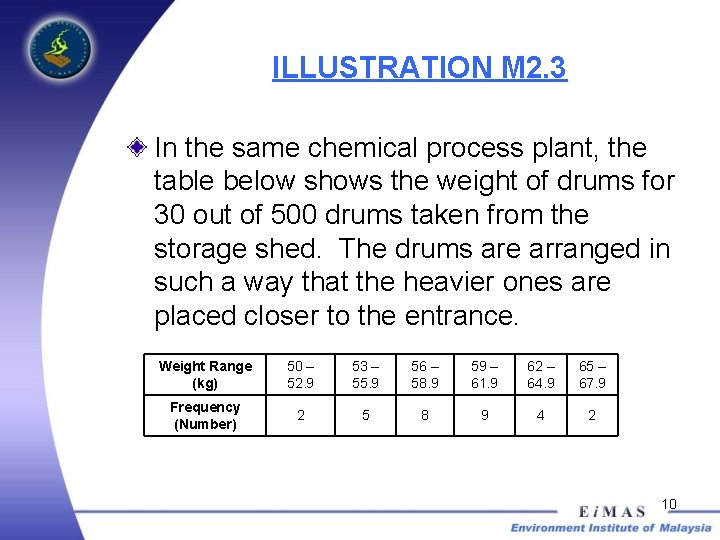
ILLUSTRATION M 2. 3 In the same chemical process plant, the table below shows the weight of drums for 30 out of 500 drums taken from the storage shed. The drums are arranged in such a way that the heavier ones are placed closer to the entrance. Weight Range (kg) 50 – 52. 9 53 – 55. 9 56 – 58. 9 59 – 61. 9 62 – 64. 9 65 – 67. 9 Frequency (Number) 2 5 8 9 4 2 10

ILLUSTRATION M 2. 3 What is the random variable for this case? Is the random variable discrete or continuous in nature? 11

ILLUSTRATION M 2. 3 What standard distribution does the graph represent? How would the shape of the curve be different if we have the weights for all the 500 drums? Suppose the 30 selected drums were sampled from those located near the entrance. How would the shape of the curve be different from the graph above? 12

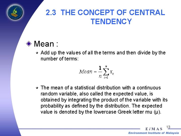
2. 3 THE CONCEPT OF CENTRAL TENDENCY Mean : Add up the values of all the terms and then divide by the number of terms: The mean of a statistical distribution with a continuous random variable, also called the expected value, is obtained by integrating the product of the variable with its probability as defined by the distribution. The expected value is denoted by the lowercase Greek letter mu (µ). 13

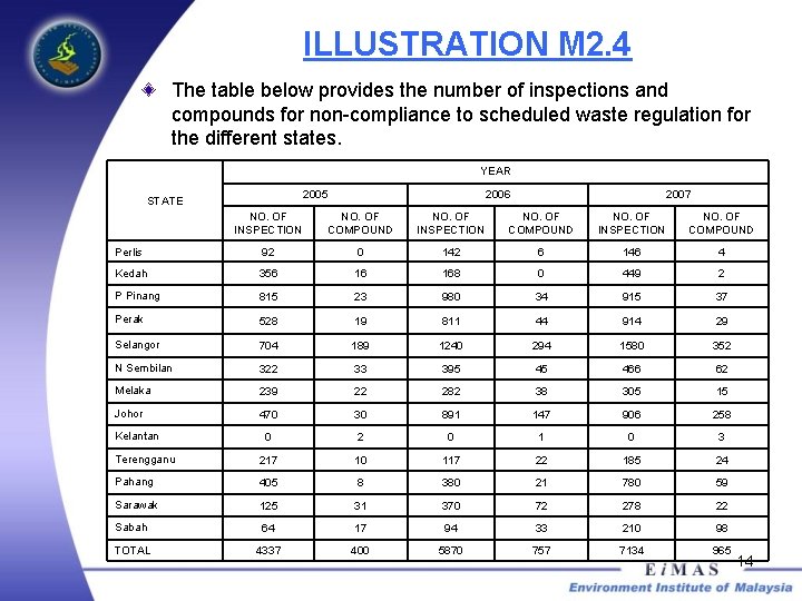
ILLUSTRATION M 2. 4 The table below provides the number of inspections and compounds for non-compliance to scheduled waste regulation for the different states. YEAR 2005 STATE 2006 2007 NO. OF INSPECTION NO. OF COMPOUND Perlis 92 0 142 6 146 4 Kedah 356 16 168 0 449 2 P Pinang 815 23 980 34 915 37 Perak 528 19 811 44 914 29 Selangor 704 189 1240 294 1580 352 N Sembilan 322 33 395 45 466 62 Melaka 239 22 282 38 305 15 Johor 470 30 891 147 906 258 0 2 0 1 0 3 Terengganu 217 10 117 22 185 24 Pahang 405 8 380 21 780 59 Sarawak 125 31 370 72 278 22 Sabah 64 17 94 33 210 98 TOTAL 4337 400 5870 757 7134 965 Kelantan 14

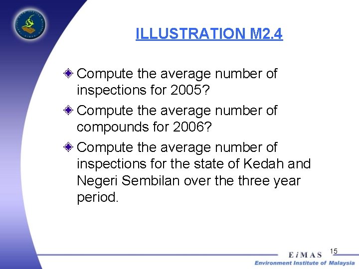
ILLUSTRATION M 2. 4 Compute the average number of inspections for 2005? Compute the average number of compounds for 2006? Compute the average number of inspections for the state of Kedah and Negeri Sembilan over the three year period. 15

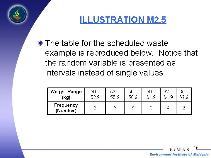
ILLUSTRATION M 2. 5 The table for the scheduled waste example is reproduced below. Notice that the random variable is presented as intervals instead of single values. Weight Range (kg) 50 – 52. 9 53 – 55. 9 56 – 58. 9 59 – 61. 9 62 – 64. 9 65 – 67. 9 Frequency (Number) 2 5 8 9 4 2 16

ILLUSTRATION M 2. 5 How can we find the mean value in this case? Compute the mean again by assuming that the frequency for each weight range has doubled. 17

2. 3 THE CONCEPT OF CENTRAL TENDENCY Median : The median of a distribution with a discrete random variable depends on whether the number of terms in the distribution is even or odd. If the number of terms is odd, then the median is the value of the term in the middle. If the number of terms is even, then the median is the average of the two terms in the middle, such that the number of terms having values greater than or equal to it is the same as the number of terms having values less than or equal to it. 18

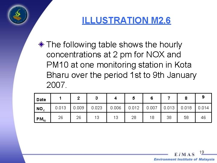
ILLUSTRATION M 2. 6 The following table shows the hourly concentrations at 2 pm for NOX and PM 10 at one monitoring station in Kota Bharu over the period 1 st to 9 th January 2007. Date 1 2 3 4 5 6 7 8 9 NOX 0. 013 0. 009 0. 023 0. 006 0. 012 0. 007 0. 013 0. 018 0. 014 PM 10 26 26 13 13 28 18 38 58 46 19

ILLUSTRATION M 2. 6 To determine the median do you need to rearrange the data? Find the median for NOX. Find the median for PM 10. Would the median for PM 10 be different if the largest value is 580 (instead of 58). Would the mean be different? What lesson can you draw from this? Suppose there are 10 days worth of observations. How would you then find the median? 20

2. 3 THE CONCEPT OF CENTRAL TENDENCY Mode : The mode of a distribution with a discrete random variable is the value of the term that occur the most often. It is not uncommon for a distribution with a discrete random variable to have more than one mode, especially if there are not many terms. The mode of a distribution with a continuous random variable is the maximum value of the function. 21

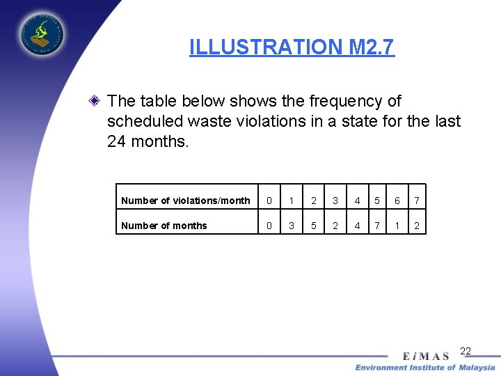
ILLUSTRATION M 2. 7 The table below shows the frequency of scheduled waste violations in a state for the last 24 months. Number of violations/month 0 1 2 3 4 5 6 7 Number of months 0 3 5 2 4 7 1 2 22

ILLUSTRATION M 2. 7 What is the random variable of interest? What is the mode for the distribution? Can you have more than one modes? Explain. What kind of statistical distribution will give you the same value for mode, mean and median? 23

2. 4 MEASURES OF DISPERSION The Range : The range R is the difference between the maximum and minimum value in the data set. This measure tends to be unstable since it depends upon the two extreme values of the data and not the entire set. The extreme values can result from exceptional observations, but the range is useful to show the extent (or limits) of the data. 24

2. 4 MEASURES OF DISPERSION The Range : In order to reduce the influence of the extreme values, inter–quartile range (IQR) is often used as indicators of the dispersion of the data. The inter-quartile range is the difference between the upper quartile and the lower quartile. The inter-quartile range gives the spread of the middle 50% of the data. 25

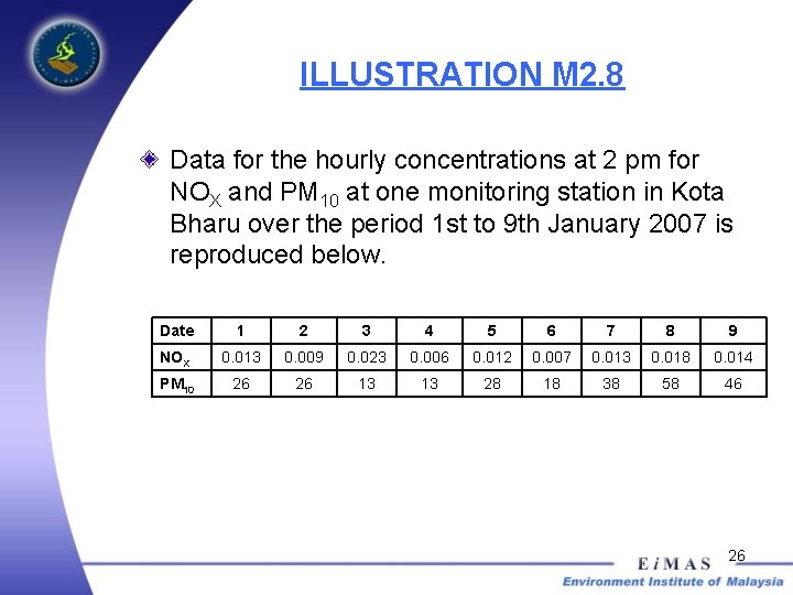
ILLUSTRATION M 2. 8 Data for the hourly concentrations at 2 pm for NOX and PM 10 at one monitoring station in Kota Bharu over the period 1 st to 9 th January 2007 is reproduced below. Date 1 2 3 4 5 6 7 8 9 NOX 0. 013 0. 009 0. 023 0. 006 0. 012 0. 007 0. 013 0. 018 0. 014 PM 10 26 26 13 13 28 18 38 58 46 26

ILLUSTRATION M 2. 8 What is the range for NOX? What is the range for PM 10? 27

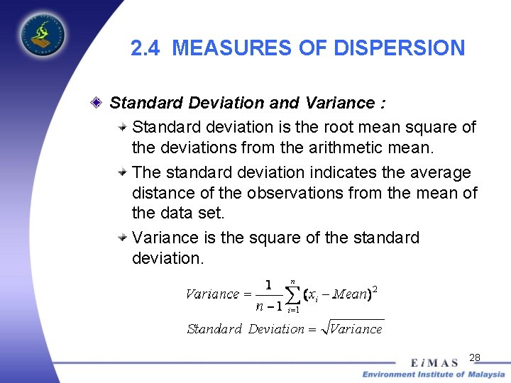
2. 4 MEASURES OF DISPERSION Standard Deviation and Variance : Standard deviation is the root mean square of the deviations from the arithmetic mean. The standard deviation indicates the average distance of the observations from the mean of the data set. Variance is the square of the standard deviation. 28

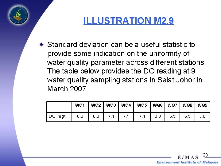
ILLUSTRATION M 2. 9 Standard deviation can be a useful statistic to provide some indication on the uniformity of water quality parameter across different stations. The table below provides the DO reading at 9 water quality sampling stations in Selat Johor in March 2007. DO, mg/l WQ 1 WQ 2 WQ 3 WQ 4 WQ 5 WQ 6 WQ 7 WQ 8 WQ 9 6. 8 7. 4 7. 1 7. 4 8. 0 6. 5 7. 8 29

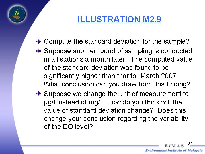
ILLUSTRATION M 2. 9 Compute the standard deviation for the sample? Suppose another round of sampling is conducted in all stations a month later. The computed value of the standard deviation was found to be significantly higher than that for March 2007. What conclusion can you draw from this finding? Suppose we change the unit of measurement to μg/l instead of mg/l. How do you think will the value of standard deviation change? Does this change your conclusion regarding the variability of the DO level? 30

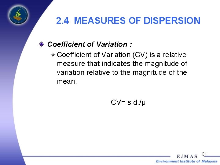
2. 4 MEASURES OF DISPERSION Coefficient of Variation : Coefficient of Variation (CV) is a relative measure that indicates the magnitude of variation relative to the magnitude of the mean. CV= s. d. /µ 31

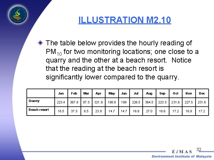
ILLUSTRATION M 2. 10 The table below provides the hourly reading of PM 10 for two monitoring locations; one close to a quarry and the other at a beach resort. Notice that the reading at the beach resort is significantly lower compared to the quarry. Jan Feb Mar Apr May Jun Jul Aug Sep Oct Nov Dec Quarry 223. 4 367. 8 87. 5 321. 8 198. 9 199 226. 5 364. 5 223. 5 231. 6 227. 5 231. 6 Beach resort 16. 5 37. 5 6. 5 23. 8 14. 7 16. 8 27. 0 16. 6 17. 2 16. 9 17. 2 32

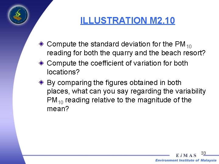
ILLUSTRATION M 2. 10 Compute the standard deviation for the PM 10 reading for both the quarry and the beach resort? Compute the coefficient of variation for both locations? By comparing the figures obtained in both places, what can you say regarding the variability PM 10 reading relative to the magnitude of the mean? 33

Managing Outliers Generally, any measurements that fall beyond the inner fences, and certainly any that fall beyond the outer fences, are considered potential outlier. Outliers are extreme measurements that stand out from the rest of the sample and may be faulty, which is incorrectly recorded observations or members of a different population from the rest of the sample. Some outliers are correct values and some are errors. If we are sure that an outlier is an error, we should correct it or delete it. If we include an outlier because we know that it is correct, we might study its effects by constructing graphs and calculated statistics with and without the outlier included. 34

2. 8 CONCLUSION This module introduces some of the more fundamental concepts in statistics under the broad categorizations of population and sample, statistical distribution, measures of central tendency and dispersion. A clear differentiation is made between the concepts of population and sample. The meaning of statistical distribution is then explained, followed by descriptions and method of computations of the measures of central tendency and dispersion. 35