Module 2 Basics of Transmission Theory and Messages

Module 2. “Basics of Transmission Theory and Messages Coding” Lecture 2. 2. CONVOLUTIONAL CODING

Convolutional code In telecommunication, a convolutional code is a type of error-correcting code in which (a) each m-bit information symbol (each m-bit string) to be encoded is transformed into an n-bit symbol, where m/n is the code rate (n ≥ m) and (b) the transformation is a function of the last k information symbols, where k is the constraint length of the code.

Where convolutional codes are used Convolutional codes are used extensively in numerous applications in order to achieve reliable data transfer, including digital video, radio, mobile communication, and satellite communication. These codes are often implemented in concatenation with a harddecision code, particularly Reed Solomon. Prior to turbo codes, such constructions were the most efficient, coming closest to the Shannon limit.

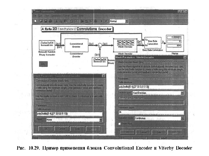
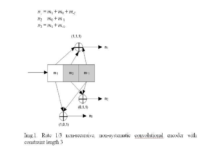
Convolutional encoding To convolutionally encode data, start with k memory registers, each holding 1 input bit. Unless otherwise specified, all memory registers start with a value of 0. The encoder has n modulo-2 adders (a modulo 2 adder can be implemented with a single Boolean XOR gate, where the logic is: 0+0 = 0, 0+1 = 1, 1+0 = 1, 1+1 = 0), and n generator polynomials — one for each adder (see figure below). An input bit m 1 is fed into the leftmost register.

Using the generator polynomials and the existing values in the remaining registers, the encoder outputs n bits. Now bit shift all register values to the right (m 1 moves to m 0, m 0 moves to m-1) and wait for the next input bit. If there are no remaining input bits, the encoder continues output until all registers have returned to the zero state. The figure below is a rate 1/3 (m/n) encoder with constraint length (k) of 3. Generator polynomials are G 1 = (1, 1, 1), G 2 = (0, 1, 1), and G 3 = (1, 0, 1). Therefore, output bits are calculated (modulo 2) as follows:

● Reed–Solomon error correction is an error-correcting code that works by oversampling (дополнительная выборка, выборка с запасом) a polynomial constructed from the data. The polynomial is evaluated at several points, and these values are sent or recorded. Sampling the polynomial more often than is necessary makes the polynomial over-determined. As long as it receives "many" of the points correctly, the receiver can recover the original polynomial even in the presence of a "few" bad points

Reed–Solomon codes are used in a wide variety of commercial applications, most prominently in CDs, DVDs and Blu-ray Discs, in data transmission technologies such as DSL & Wi. MAX, in broadcast systems such as DVB and ATSC, and in computer applications such as RAID 6 systems. Reed–Solomon codes are block codes. This means that a fixed block of input data is processed into a fixed block of output data. In the case of the most commonly used R–S code (255, 223) – 223 Reed–Solomon input symbols (each eight bits long) are encoded into 255 output symbols.

- Most R–S error-correcting code schemes are systematic. This means that some portion of the output codeword contains the input data in its original form. - A Reed–Solomon symbol size of eight bits forces the longest codeword length to be 255 symbols. - The standard (255, 223) Reed–Solomon code is capable of correcting up to 16 Reed–Solomon symbol errors in each codeword. Since each symbol is actually eight bits, this means that the code can correct up to 16 short bursts of error.

The Reed–Solomon code, like the convolutional code, is a transparent code. This means that if the channel symbols have been inverted somewhere along the line, the decoders will still operate. The result will be the complement (дополнение) of the original data. However, the Reed–Solomon code loses its transparency when the code is shortened (see below). The "missing" bits in a shortened code need to be filled by either zeros or ones, depending on whether the data is complemented or not. (To put it another way, if the symbols are inverted, then the zero fill needs to be inverted to a ones fill. ) For this reason it is mandatory that the sense of the data (i. e. , true or complemented) be resolved before Reed–Solomon decoding.

The key idea behind a Reed–Solomon code is that the data encoded is first visualized as a polynomial. The code relies on a theorem from algebra that states that any k distinct points uniquely determine a univariate polynomial of degree, at most, k − 1. The sender determines a degree k − 1 polynomial, over a finite field, that represents the k data points. The polynomial is then "encoded" by its evaluation at various points, and these values are what is actually sent. During transmission, some of these values may become corrupted. Therefore, more than k points are actually sent. As long as sufficient values are received correctly, the receiver can deduce what the original polynomial was, and hence decode the original data. In the same sense that one can correct a curve by interpolating past a gap, a Reed–Solomon code can bridge a series of errors in a block of data to recover the coefficients of the polynomial that drew the original curve.

Cryptographic Hash Functions and their many applications

What are hash functions? • Just a method of compressing strings – E. g. , H : {0, 1}* {0, 1}160 – Input is called “message”, output is “digest” • Why would you want to do this? – Short, fixed-size better than long, variable-size • True also for non-crypto hash functions – Digest can be added for redundancy – Digest hides possible structure in message

How are they built? But not always… Typically using Merkle-Damgård iteration: 1. Start from a “compression function” – h: {0, 1}b+n {0, 1}n |M|=b=512 bits c =160 bits h d=h(c, M)=160 bits 2. Iterate it M 1 IV=d 0 M 2 h d 1 ML-1 h d 2 … ML h d. L-1 h d. L d=H(M)

What are they good for? “Modern, collision resistant hash functions were designed to create small, fixed size message digests so that a digest could act as a proxy for a possibly very large variable length message in a digital signature algorithm, such as RSA or DSA. These hash functions have since been widely used for many other “ancillary” applications, including hash-based message authentication codes, pseudo random number generators, and key derivation functions. ” “Request for Candidate Algorithm Nominations”, -- NIST, November 2007

Some examples • • • Signatures: sign(M) = RSA-1( H(M) ) Message-authentication: tag=H(key, M) Commitment: commit(M) = H(M, …) Key derivation: AES-key = H(DH-value) Removing interaction [Fiat-Shamir, 1987] – Take interactive identification protocol – Replace one side by a hash function Challenge = H(smthng, context) – Get non-interactive signature scheme A smthng B challenge response smthng, response

Part I: Random functions vs. hash functions

Random functions • What we really want is H that behaves “just like a random function”: Digest d=H(M) chosen uniformly for each M – Digest d=H(M) has no correlation with M – For distinct M 1, M 2, …, digests di=H(Mi) are completely uncorrelated to each other – Cannot find collisions, or even near-collisions – Cannot find M to “hit” a specific d – Cannot find fixed-points (d = H(d)) – etc.

The “Random-Oracle paradigm” [Bellare-Rogaway, 1993] 1. Pretend hash function is really this good 2. Design a secure cryptosystem using it § Prove security relative to a “random oracle”

The “Random-Oracle paradigm” [Bellare-Rogaway, 1993] 1. Pretend hash function is really this good 2. Design a secure cryptosystem using it § Prove security relative to a “random oracle” 3. Replace oracle with a hash function § Hope that it remains secure

The “Random-Oracle paradigm” [Bellare-Rogaway, 1993] 1. Pretend hash function is really this good 2. Design a secure cryptosystem using it § Prove security relative to a “random oracle” 3. Replace oracle with a hash function § Hope that it remains secure • Very successful paradigm, many schemes – E. g. , OAEP encryption, FDH, PSS signatures • Also all the examples from before… – Schemes seem to “withstand test of time”

Random oracles: rationale • S is some crypto scheme (e. g. , signatures), that uses a hash function H • S proven secure when H is random function Any attack on real-world S must use some “nonrandom property” of H • We should have chosen a better H – without that “nonrandom property” • Caveat: how do we know what “nonrandom properties” are important?

This rationale isn’t sound [Canetti-Goldreich-H 1997] • Exist signature schemes that are: 1. Provably secure wrt a random function 2. Easily broken for EVERY hash function • Idea: hash functions are computable – This is a “nonrandom property” by itself • Exhibit a scheme which is secure only for “non-computable H’s” – Scheme is (very) “contrived”

Contrived example • Start from any secure signature scheme – Denote signature algorithm by SIG 1 H(key, msg) • Change SIG 1 to SIG 2 as follows: Some Technicalities SIG 2 H(key, msg): interprate msg as code P – If P(i)=H(i) for i=1, 2, 3, …, |msg|, then output key – Else output the same as SIG 1 H(key, msg) • If H is random, always the “Else” case • If H is a hash function, attempting to sign the code of H outputs the secret key

Cautionary note • ROM proofs may not mean what you think… – Still they give valuable assurance, rule out “almost all realistic attacks” • What “nonrandom properties” are important for OAEP / FDH / PSS / …? • How would these scheme be affected by a weakness in the hash function in use? • ROM may lead to careless implementation

Merkle-Damgård vs. random functions h h … h • Recall: we often construct our hash functions from compression functions – Even if compression is random, hash is not • E. g. , H(key|M) subject to extension attack – H(key | M|M’) = h( H(key|M), M’) – Minor changes to MD fix this • But they come with a price (e. g. prefix-free encoding) • Compression also built from low-level blocks – E. g. , Davies-Meyer construction, h(c, M)=EM(c) c – Provide yet more structure, can lead to attacks on provable ROM schemes [H-Krawczyk 2007] h

Part II: Using hash functions in applications

Using “imperfect” hash functions • Applications should rely on “specific security properties” of hash functions – Try to make these properties as “standard” and as weak as possible • Increases the odds of long-term security – When weaknesses are found in hash function, application more likely to survive – E. g. , MD 5 is badly broken, but HMAC-MD 5 is barely scratched

Security requirements • Deterministic hashing Stronger – Attacker chooses M, d=H(M) • Hashing with a random salt – Attacker chooses M, then good guy chooses public salt, d=H(salt, M) • Hashing random messages – M random, d=H(M) • Hashing with a secret key – Attacker chooses M, d=H(key, M) Weaker

Deterministic hashing • Collision Resistance – Attacker cannot find M, M’ such that H(M)=H(M’) • Also many other properties – Hard to find fixed-points, near-collisions, M s. t. H(M) has low Hamming weight, etc.

Hashing with public salt • Target-Collision-Resistance (TCR) – Attacker chooses M, then given random salt, cannot find M’ such that H(salt, M)=H(salt, M’) • enhanced TRC (e. TCR) – Attacker chooses M, then given random salt, cannot find M’, salt’ s. t. H(salt, M)=H(salt’, M’)

Hashing random messages • Second Preimage Resistance – Given random M, attacker cannot find M’ such that H(M)=H(M’) • One-wayness – Given d=H(M) for random M, attacker cannot find M’ such that H(M’)=d • Extraction* – For random salt, high-entropy M, the digest d=H(salt, M) is close to being uniform * Combinatorial, not cryptographic

Hashing with a secret key • Pseudo-Random Functions – The mapping M H(key, M) for secret key looks random to an attacker • Universal hashing* – For all M M’, Prkey[ H(key, M)=H(key, M’) ]<e * Combinatorial, not cryptographic

Application 1: Digital signatures • Hash-then-sign paradigm – First shorten the message, d = H(M) – Then sign the digest, s = SIGN(d) • Relies on collision resistance – If H(M)=H(M’) then s is a signature on both Attacks on MD 5, SHA-1 threaten current signatures – MD 5 attacks can be used to get bad CA cert [Stevens et al. 2009]

Collision resistance is hard • Attacker works off-line (find M, M’) – Can use state-of-the-art cryptanalysis, as much computation power as it can gather, without being detected !! • Helped by birthday attack (e. g. , 280 vs 2160) • Well worth the effort – One collision forgery for any signer

Signatures without CRHF [Naor-Yung 1989, Bellare-Rogaway 1997] • Use randomized hashing – To sign M, first choose fresh random salt – Set d= H(salt, M), s= SIGN( salt || d ) • Attack scenario (collision game): – Attacker chooses M, M’ same salt (since salt is explicitly signed) – Signer chooses random salt – Attacker must find M' s. t. H(salt, M) = H(salt, M') • Attack is inherently on-line – Only rely on target collision resistance

TCR hashing for signatures • Not every randomization works – H(M|salt) may be subject to collision attacks • when H is Merkle-Damgård – Yet this is what PSS does (and it’s provable in the ROM) • Many constructions “in principle” – From any one-way function • Some engineering challenges – Most constructions use long/variable-size randomness, don’t preserve Merkle-Damgård • Also, signing salt means changing the underlying signature schemes

Signatures with enhanced TCR [H-Krawczyk 2006] • Use “stronger randomized hashing”, e. TCR – To sign M, first choose fresh random salt – Set d = H(salt, M), s = SIGN( d ) • Attack scenario (collision game): – Attacker chooses M attacker can use different salt’ – Signer chooses random salt – Attacker needs M‘, salt’ s. t. H(salt, M)=H(salt', M') • Attack is still inherently on-line

Randomized hashing with RMX [H-Krawczyk 2006] • Use simple message-randomization – RMX: M=(M 1, M 2, …, ML), r (r, M 1 r, M 2 r, …, ML r) • Hash( RMX(r, M) ) is e. TCR when: – Hash is Merkle-Damgård, and – Compression function is ~ 2 nd-preimage-resistant • Signature: [ r, SIGN( Hash( RMX(r, M) )) ] – r fresh per signature, one block (e. g. 512 bits) – No change in Hash, no signing of r

Preserving hash-then-sign M =(M 1, …, ML) RMX r (r, M 1 r, , …, ML r) HASH TCR SIGN X

Application 2: Message authentication • Sender, Receiver, share a secret key • Compute an authentication tag – tag = MAC(key, M) • Sender sends (M, tag) • Receiver verifies that tag matches M • Attacker cannot forge tags without key

Authentication with HMAC [Bellare-Canetti-Krawczyk 1996] 1996 • Simple key-prepend/append have problems when used with a Merkle-Damgård hash – tag=H(key | M) subject to extension attacks – tag=H(M | key) relies on collision resistance • HMAC: Compute tag = H(key | M)) – About as fast as key-prepend for a MD hash • Relies only on PRF quality of hash – M H(key|M) looks random when key is secret

Authentication with HMAC [Bellare-Canetti-Krawczyk 1996] 1996 • Simple key-prepend/append have problems when used with a Merkle-Damgård hash – tag=H(key subject barely to extension attacks As| M) a result, – tag=H(Maffected | key) relies collision resistance by on collision attacks • HMAC: Compute tag = on H(key | M)) – About as fast. MD 5/SHA 1 as key-prepend for a MD hash • Relies only on PRF property of hash – M H(key|M) looks random when key is secret

Carter-Wegman authentication [Wegman-Carter 1981, …] 1981, … • Compress message with hash, t=H(key 1, M) • Hide t using a PRF, tag = t PRF(key 2, nonce) – PRF can be AES, HMAC, RC 4, etc. – Only applied to a short nonce, typically not a performance bottleneck • Secure if the PRF is good, H is “universal” – For M M’, D, Prkey[ H(key, M) H(key, M’)=D ]<e) – Not cryptographic, can be very fast

Fast Universal Hashing • “Universality” is combinatorial, provable no need for “security margins” in design • Many works on fast implementations From inner-product, Hk 1, k 2(M 1, M 2)=(K 1+M 1)·(K 2+M 2) • [H-Krawczyk’ 97, Black et al. ’ 99, …] From polynomial evaluation Hk(M 1, …, ML)=Si Mi ki • [Krawczyk’ 94, Shoup’ 96, Bernstein’ 05, Mc. Grew-Viega’ 06, …] • As fast as 2 -3 cycle-per-byte (for long M’s) – Software implementation, contemporary CPUs

Part III: Designing a hash function Fugue: IBM’s candidate for the NIST hash competition

Design a compression function? h h … h h PROs: modular design, reduce to the “simpler problem” of compressing fixed-length strings – Many things are known about transforming compression into hash CONs: compression hash has its problems – It’s not free (e. g. message encoding) – Some attacks based on the MD structure • Extension attacks ( rely on H(x|y)=h(H(x), y) ) • “Birthday attacks” (herding, multicollisions, …)

Example attack: herding [Kelsey-Kohno 2006] • Find many off-line collisions – “Tree structure” with ~2 n/3 di, j’s – Takes ~ 22 n/3 time • Publish final d • Then for any prefix P M 1, 1 d 1, 1 h M 1, 2 h d 1, 2 M 2, 1 d 2, 1 h M 1, 3 h d 1, 3 M 1, 4 d h – Find “linking block” L s. t. H(P|L) in the tree – Takes ~ 22 n/3 time – Read off the tree the suffix S to get to d Show an extension of P s. t. H(P|L|S) = d M 2, 2 d 2, 2 h

The culprit: small intermediate state • With a compression function, we: – Work hard on current message block – Throw away this work, keep only n-bit state • Alternative: keep a large state – Work hard on current message block/word – Update some part of the big state • More flexible approach – Also more opportunities to mess things up

The hash function Grindahl [Knudsen-Rechberger-Thomsen 2007] 2007 • State is 13 words = 52 bytes • Process one 4 -byte word at a time – One AES-like mixing step per word of input • After some final processing, output 8 words • Collision attack by Peyrin (2007) – Complexity ~ 2112 (still better than brute-force) • Recently improved to ~ 2100 [Khovratovich 2009] – “Start from a collision and go backwards”

The hash function “Fugue” [H-Hall-Jutla 2008] • Proof-driven design – Designed to enable analysis Proofs that Peyrin-style attacks do not work • State of 30 4 -byte words = 120 bytes • Two “super-mixing” rounds per word of input – Each applied to only 16 bytes of the state – With some extra linear diffusion • Super-mixing is AES-like – But uses stronger MDS codes

Fugue-256 Initial State (30 words) Process M 1 New State Iterate State Final Processing Output 8 words = 256 bits Mi

Collision attacks Initial State (30 words) Process Think of M 1, …, ML and M’ 1, …, M’L DM 1 New State Iterate D State= 0? Final Processing D=0 DMi Collision means that DMi’s are not all zero D State = 0 Internal collision D State 0 External collision

Processing one input word Initial State (30 words) 1. Input one word Process M 1 2. Shift 3 columns to right 3. XOR into columns 1 -3 4. “super-mix” operation on columns 1 -4 This is where the crypto happens M 1 SMIX New State Process Repeat 2 -4 once more Iterate State Final Stage

SMIX in Fugue • Similar to one AES round – Works on a 4 x 4 matrix of bytes – Starts with S-box substitution • Byte b, S[256] = {. . . }; . . . • b = S[b]; – Does linear mixing • Stronger mixing than AES – Diagonal bytes as in AES – Other bytes are mixed into both column and row

SMIX in Fugue • In algebraic notation: b'1 b'2 M b'16 = M 16 x 16 S[b 1] S[b 2] M S[b 16] • M generates a good linear code – If all the bi’ bytes but 4 are zero then 13 of the S[bi] bytes must be nonzero – And other such properties

Analyzing internal collisions* now D 28 -1 0 3 columns still D 1 -4 0 before SMIX: D 1 -4 0 4 nonzero SMIX byte diffs before input word: D 1 0 D After last input word: DState=0 * a bit oversimplified

Analyzing internal collisions* D 25 -1 0 3 columns D 28 -4 0 4 nonzero SMIX byte diffs now D 28 -1 0 3 columns still D 1 -4 0 before SMIX: D 1 -4 0 before input word: D 1 0 SMIX D after input word: DState=0 * a bit oversimplified

Analyzing internal collisions* before input: D 1=? , D 25 -30 0 D’ D 25 -1 0 3 columns D 28 -4 0 SMIX now D 28 -1 0 3 columns still D 1 -4 0 before SMIX: D 1 -4 0 before input word: D 1 0 SMIX D after input word: DState=0 * a bit oversimplified

Many nonzero byte differences before the SMIX operations The analysis from previous slides was upto here

Analyzing internal collisions • What does this mean? Consider this attack: – Attacker feeds in random M 1, M 2, … and M’ 1, M’ 2, … – Until State. L State’L = some “good D” – Then it searches for suffixed (ML+1, …, ML+4), (M’L+1, …, M’L+4) that will induce internal collision Theorem*: For any fixed D, Pr[ suffixes that induce collision ] < 2 -150 * Relies on a very mild independence assumptions

Analyzing internal collisions • Why do we care about this analysis? • Peyrin’s attacks are of this type • All differential attacks can be seen as (optimizations of) this attack – Entities that are not controlled by attack are always presumed random • A known “collision trace” is as close as we can get to understanding collision resistance

Fugue: concluding remarks • Similar analysis also for external collisions – “Unusually thorough” level of analysis • Performance comparable to SHA-256 – But more amenable to parallelism • One of 14 submissions that were selected by NIST to advance to 2 nd round of the SHA 3 competition

Morals • Hash functions are very useful • We want them to behave “just like random functions” – But they don’t really • Applications should be designed to rely on “as weak as practical” properties of hashing – E. g. , TCR/e. TCR rather than collision-resistance • A taste of how a hash function is built

Thank you!

END