Module 1 Review of descriptive statistics hypothesis testing

Module 1 Review of descriptive statistics, hypothesis testing and SPSS Wei Metropolitan State University Saint Paul, Minnesota, USA

Learning objectives and outcomes • Understand descriptive statistics • Know how to use SPSS to calculate descriptive statistics • Know how to use SPSS to generate graphs • Know how to use descriptive statistics and graphs to explore data

What is statistics? • Discussion – How to prove “lung cancer and smoking are related”?

What is statistics? • Definition: Statistics is the science of planning studies and experiments; obtaining data; summarizing data; analyzing data; and draw conclusions • Steps: – Prepare: Have a goal of study and Take samples – Analyze: Analyze data – Conclude: Draw a conclusion based on your analysis results

Population vs. Sample • Population: all individuals that are being considered • Sample: Subcollection of members selected from a population • Individual (or subject): objects described by a data; can be people, cars, animals etc. Individual Population Sample

Parameter vs. Statistic • Parameter: numerical measurement for a population; – something for “all” • Statistic: numerical measurement for a sample; – something for a “sample”

Parameter vs. Statistic – We would like to examine the birth weight of new born infants in the U. S. The average birth weight of all infants is 6. 8 lbs. What is the 6. 8? • A) Parameter • B) Statistic

Data Type • Categorical data: names or labels that place an individual into one of the several categories – Example: Gender (male, female) – Note: sometimes a categorical data is represented by numbers, but the difference of two values does not make sense • Example: Gender (1, 2) • Numeric data: numbers representing counts or measurements – Example: birth weight; height

Data Type • Categorical data: – Nominal data: The data cannot be arranged in an order – Example: Gender (male, female); Marital Status (single, married); Hair color (black, brown, blonde, red) – Ordinal data: The data can be arranged in some order – Example: 今天的空气质量（非常好，一般，不好， 很糟）Students’ final letter grades (A, B, C, D, F)

Data Type • Numeric – Discrete: Countable integers – Example: The number of children in a family; The number of steps for a stair; The number of students sleeping in a stat class – Continuous: Any number in an interval – Example: height (in cm); Time to wake up a sleeping student

Data Type • Activity/ Discussion A researcher wishes to know the type of car each person drives in the United States. So he gets permission to go to the student parking lot at a college and record some data. He then made a spreadsheet that includes each car’s model, color, level of damage, weight and number of cylinders. a) What is the population? What is the sample? b) Describe the data type for each variable: model, color, level of damage, weight and # of cylinders

Observational study vs. Experiment • Definition: – Observational Study: observe and measure specific characteristics, but don’t apply treatments to the subjects – Experiment: apply treatments to the subjects and observe the effects

Observational study vs. Experiment • Discussion: – In a clinical trial study, the nurses measured the 100 participants’ blood pressure every year, calculated the average and compared among different years – Researchers would like to study whether or not dark chocolate can help improving blood flow. Researchers fed a small 1. 6 ounce bar of chocolate to each of 22 volunteers daily for two weeks. Half of the subjects were randomly assigned to receive dark chocolate, and the other half received milk chocolate. Researchers tested whether the average blood flow is higher for those who took dark chocolate. – 消失的弹孔

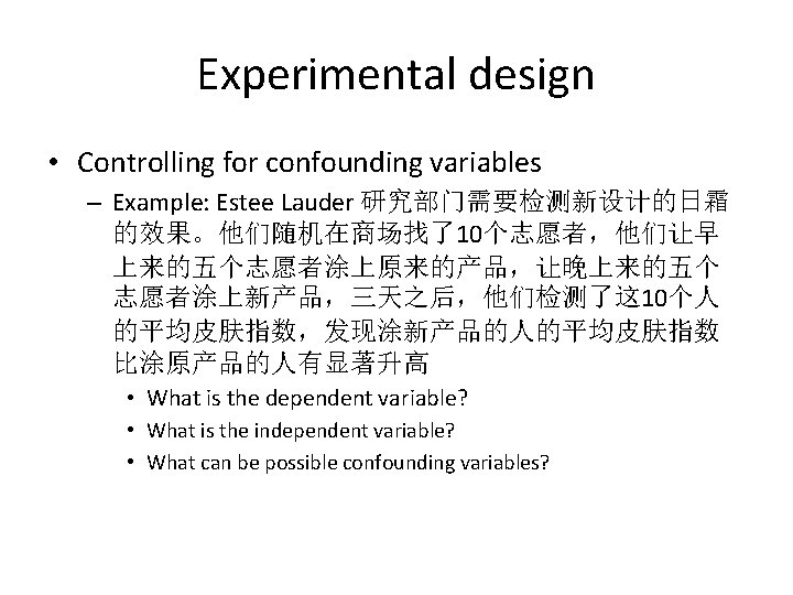
Explanatory variable and response variable Definition of response variable: A response variable, y, also called the dependent variable, is the variable that shows the outcome of a study or an experiment. It is usually what the researchers record, measure or test at the end of the study. Definition of explanatory variable: An explanatory variable, x, also called the independent variable, is the variable that explains the cause of difference in the dependent variable values. Definition of confounding variable: A variable that can potentially cause different responses in the dependent variable, but not of the research interest

Explanatory and response variables • Example: – Researchers would like to study whether or not dark chocolate can help improving blood flow. Researchers fed a small 1. 6 ounce bar of chocolate to each of 22 volunteers daily for two weeks. Half of the subjects were randomly assigned to receive dark chocolate, and the other half received milk chocolate. Researchers tested whether the average blood flow is higher for those who took dark chocolate. – What is the explanatory variable? – What is the response variable?

Explanatory and response variables • Discussion Four cough formulas are compared in an experiment, with the variable measured being hours to relief from coughing. Data are shown in the table. Twenty patients were selected into the experiment. Five of them took formula 1 and the hours to relief were recorded under column A. Five of them took formula 2 and the hours to relief were recorded under column B. Five of them took formula 3 and five took formula 4, and the time to relief for those two groups were recorded under column 3 and 4. Do these cough formulas have the same mean hours to relief? Perform a test to support your answer based on the significance level of 0. 05.

Experimental Design • Experimental design and analysis are interrelated • Before you collect data, you should be clear about the following: – The research question (goal of the study) – The dependent and independent variables – What types of data will you collect? (Dependent and independent variable type) – Determine approximate sample size

Experimental design • Dealing with confounding variables – Decide possible confounding variables – Decide how to best to control them – If can’t control the major ones, need to count them in the analysis

Arithmetic Mean •

Arithmetic Mean • Example: A sample of four liv-born infants was taken at a hospital in San Diego, CA. The birth weights, in g, were measured for these babies and recorded in the following table. What is the mean birth weight of the 6 infants? Individual (i) 1 2 3 4 5 6 3265 3260 3245 3484 4146 3323

Median •

Median • Example (continue with the birth weight example): What is the median birth weight of the 6 infants? Individual (i) 1 2 3 4 5 6 3265 3260 3245 3484 4146 3323

Outlier effects on mean and median •

Mode • Definition: the mode is the most frequently occurring value among all the observations. • Example: Consider the sample of time intervals between successive menstrual periods, in days, for a group of 451 women shown in the table. What is the mode? Menstrual period (days) 25 26 27 28 29 30 Frequency 10 28 64 185 96 63

Quartiles/percentiles • Definition of pth percentile: p% of the observations are smaller than it • Definition of 1 st quartile (25 th percentile): 25% of the observations are smaller than the 1 st quartile; the median of the observations below the overall median • Definition of 3 rd quartile (75 th percentile): 75% of the observations are smaller than the 3 rd quartile; the median of the observations above the overall median

Quartiles/percentiles • Example (cont. ) What is the 1 st quartile of the birth weight of the 6 infants? What is the 3 rd quartile? Individual (i) 1 2 3 4 5 6 3265 3260 3245 3484 4146 3323

Range •

Standard deviation & Variance •

Standard deviation and variance • Example (cont. ) What is the standard deviation of the birth weight of 6 infants? What is the variance? Individual (i) 1 2 3 4 5 6 3265 3260 3245 3484 4146 3323

How to enter data into SPSS Example: We would like to enter the following data into SPSS. The data shows the record of the 6 infants including name, gender and birth weight. Enter the data into SPSS and save the data Name Gender Birth weight Jason Male 3265 Jerry Male 3260 Emily Female 3245 Tina Female 3484 Jayden Male 4146 Emma Female 3323

How to enter data into SPSS • Columns are variables; Rows are individuals a) Click “Variable view” and enter the three variables: “name” and “gender” as a string with the default width (8 characters); “birth weight” as a scale with the default width. Save the data as “birth weight data” Note: variable name can not contain “space” and should be <12 characters; “birth_weight” will work

Show descriptive statistics in SPSS • • • Analyze->Descriptive statistics->Explore Move the variable to the “dependent list” Click “statistics” check “descriptive” OK Output – Mean – 95% confidence interval of the mean – Range – Median – Variance, standard deviation

Scatter plot in SPSS • Scatter plot shows the relationship between two variables, x and y (IV and DV) • Graphs->Legacy Dialogs->Scatter plot->Simple Scatter plot • Choose the x and y variables; Choose a title for the graph • If you want to edit the graph, double click the graph

Scatter plot • Example: • Generate a scatter plot for the data on d 2 l “Birth and Mortality”; • Use your scatter plot to answer the question “Is there a correlation between birth rate and mortality rate for these countries? ”

Activity graph • There is a correlation between birth rate and mortality rate; When birth rate is increasing, the mortality rate is decreasing

Box plot • A box plot of a numeric variable shows the five number summary – Median – Minimum – Maximum – 1 st quartile – 3 rd quartile AND – outliers • Graphs->Legacy Dialogs->Boxplot->Simple • Choose your Variable (DV) and Category Axis (IV)

Box plot Maximum 3 rd quartile (75 th percentile) Median 1 st quartile (25 th percentile) Minimum

Box plot • Example: The data “PDI data ” on d 2 l recorded Psychomotor Development Index (PDI scores, 运动发育指数) for 143 infants underwent two types of treatments (0: Circulatory arrest 循 环停止; 1: Low-flow bypass 低流量体外循环 ). Make a box plot to compare the PDI scores after the two treatments; Which treatment leads to higher PDI score? IS there any outliers?

Activity graph • Treatment 1 (Low-flow by pass) has a higher median PDI score; The individual 118, 141 and 85 are outliers for treatment 1.

Bar Graph in SPSS • Bar graph can show – Means for numeric variables – Frequencies for categorical variables • Graphs->Legacy Dialogs->Bar>Simple • Choose the Category Axis (IV) and Variable (DV) – If the bar graph is not for frequency (N) or relative frequency (%), then choose “other statistics” – Choose your statistic to be shown • Example: Use the PDI data, generate the bar graph to show the average PDI scores for the two treatments

Activity graph • The low-flow bypass treatment has a higher average PDI score