Module 1 An Overview of Operating System Subject

Module 1 An Overview of Operating System Subject Name: Machine Learning Subject Code: 15 EC 834 Dr P KARTHIK Professor K. S. SCHOOL OF ENGINEERING AND MANAGEMENT, BANGALORE 560109 DEPARTMENT OF ELETRONICS AND COMMUNICATION ENGINEERING

Introduction • Ever since computers were invented, we have wondered whether they might be made to learn. If we could understand how to program them to learn-to improve automatically with experience, the impact would be dramatic. • Imagine computers learning from medical records which treatments are most effective for new diseases or personal software assistants learning the evolving interests of their users in order to highlight especially relevant stories from the online morning newspaper.

Successful applications of machine learning are: • Learning to recognize spoken words. • Learning to drive an autonomous vehicle. • Learning to classify new astronomical structures. • Learning to play world-class games.

Well Posed Learning Problems Definition: A computer program is said to learn from experience E with respect to some class of tasks T and performance measure P, if its performance at tasks in T, as measured by P, improves with experience E.

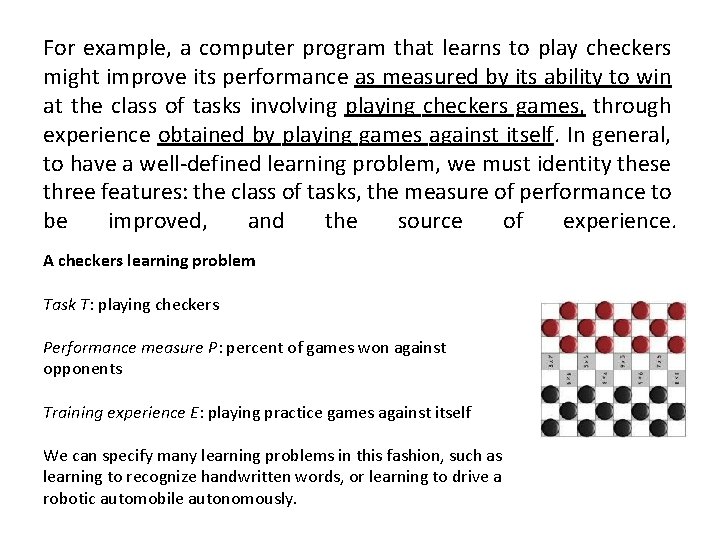
For example, a computer program that learns to play checkers might improve its performance as measured by its ability to win at the class of tasks involving playing checkers games, through experience obtained by playing games against itself. In general, to have a well-defined learning problem, we must identity these three features: the class of tasks, the measure of performance to be improved, and the source of experience. A checkers learning problem Task T: playing checkers Performance measure P: percent of games won against opponents Training experience E: playing practice games against itself We can specify many learning problems in this fashion, such as learning to recognize handwritten words, or learning to drive a robotic automobile autonomously.

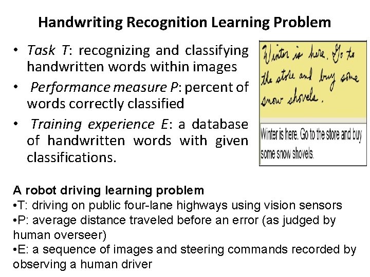
Handwriting Recognition Learning Problem • Task T: recognizing and classifying handwritten words within images • Performance measure P: percent of words correctly classified • Training experience E: a database of handwritten words with given classifications. A robot driving learning problem • T: driving on public four-lane highways using vision sensors • P: average distance traveled before an error (as judged by human overseer) • E: a sequence of images and steering commands recorded by observing a human driver

Designing a Learning System In order to illustrate some of the basic design issues and approaches to machine learning, let us consider designing a program to learn to play checkers, with the goal of entering it in the world checkers tournament. We adopt the obvious performance measure: the percent of games it wins in this world tournament.

Choosing the Training Experience • The type of training experience available can have a significant impact on success or failure of the learner. • One key attribute is whether the training experience provides direct or indirect feedback regarding the choices made by the performance system. • For example, in learning to play checkers, the system might learn from direct training examples consisting of individual checkers board states and the correct move for each. • Alternatively, it might have available only indirect information consisting of the move sequences and final outcomes of various games played. Here the learner faces an additional problem of credit assignment or determining the degree to which each move in the sequence deserves credit or blame for the final outcome. Hence, learning from direct training feedback is typically easier than learning from indirect feedback.

• A second important attribute of the training experience is the degree to which the learner controls the sequence of training examples. For example, the learner might rely on the teacher to select informative board states and to provide the correct move for each. Alternatively, the learner might itself propose board states that it finds particularly confusing and ask the teacher for the correct move. • A third important attribute of the training experience is how well it represents the distribution of examples over which the final system performance P must be measured.

Choosing the Target Function • A function that chooses the best move M for any B – Choose. Move : B --> M – Difficult to learn • It is useful to reduce the problem of improving performance P at task T to the problem of learning some particular target function. • An evaluation function that assigns a numerical score to any B V : B --> R

An alternative target function and one that will turn out to be easier to learn in this setting is an evaluation function that assigns a numerical score to any given board state. Let us call this target function V and again use the notation V: B → M to denote that V maps any legal board state from the set B to some real value in M. We intend for this target function V to assign higher scores to better board states. If the system can successfully learn such a target function V, then it can easily use it to select the best move from any current board position. This can be accomplished by generating the successor board state produced by every legal move, then using V to choose the best successor state and therefore the best legal move. For example, define the target value V(b) for an arbitrary board state b in B, as follows: if b is a final board state that is won, then V(b) = 100 if b is a final board state that is lost, then V(b) = -100 if b is a final board state that is drawn, then V(b) = 0 if b is a not a final state in the game, then V(b) = V(b'), where b' is the best final board state that can be achieved starting from b and playing optimally until the end of the game (assuming the opponent plays optimally, as well). While this recursive definition specifies a value of V(b) for every board state b, this definition is not usable by our checkers player because it is not efficiently computable. The goal of learning in this case is to discover an operational description of V; i. e. select moves within realistic time bounds. Thus, we have reduced the learning task in this case to the problem of discovering an operational description of the ideal target function V.

Choosing a Representation for the Target Function • We have several ways to represent like; using a large table with a distinct entry specifying the value for each distinct board state or using a collection of rules that match against features of the board state, or a quadratic polynomial function of predefined board features, or an artificial neural network. • On the other hand, the more expressive the representation, the more training data the program will require in order to choose among the alternative hypotheses it can represent. To keep the discussion brief, let us choose a simple representation: for any given board state, the function c will be calculated as a linear combination of the following board features:

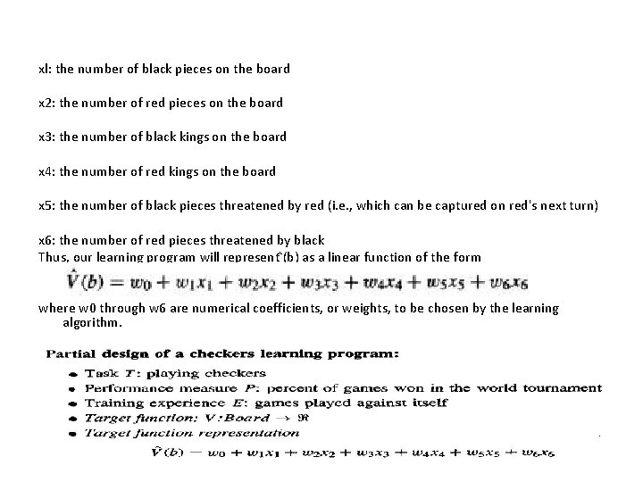
xl: the number of black pieces on the board x 2: the number of red pieces on the board x 3: the number of black kings on the board x 4: the number of red kings on the board x 5: the number of black pieces threatened by red (i. e. , which can be captured on red's next turn) x 6: the number of red pieces threatened by black Thus, our learning program will represent (b) as a linear function of the form where w 0 through w 6 are numerical coefficients, or weights, to be chosen by the learning algorithm.

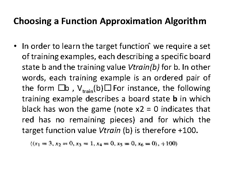
Choosing a Function Approximation Algorithm • In order to learn the target function we require a set of training examples, each describing a specific board state b and the training value Vtrain(b) for b. In other words, each training example is an ordered pair of the form �b , Vtrain(b)�. For instance, the following training example describes a board state b in which black has won the game (note x 2 = 0 indicates that red has no remaining pieces) and for which the target function value Vtrain (b) is therefore +100.

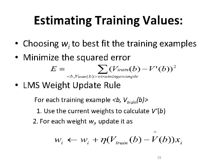
Estimating Training Values: • Choosing wi to best fit the training examples • Minimize the squared error • LMS Weight Update Rule For each training example <b, Vtrain(b)> 1. Use the current weights to calculate V’(b) 2. For each weight wi, update it as 15

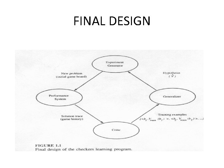
FINAL DESIGN

Concept of Concepts • Examples of Concepts – “birds”, “car”, “situations in which I should study more in order to pass the exam” • Concept – Some subset of objects or events defined over a larger set, or – A boolean-valued function defined over this larger set. – Concept “birds” is the subset of animals that constitute birds.

Perspective and Issues in Machine Learning • One useful perspective on machine learning is that it involves searching a very large space of possible hypotheses to determine one that best fits the observed data and any prior knowledge held by the learner. • Issues in ML - Our checkers example raises a number of generic questions about machine learning. The field of machine learning, is concerned with answering questions like

• What algorithms exist for learning general target functions from specific training examples? In what settings will particular algorithms converge to the desired function, given sufficient training data? Which algorithms perform best for which types of problems and representations? • • How much training data is sufficient? What general bounds can be found to relate the confidence in learned hypotheses to the amount of training experience and the character of the learner's hypothesis space?

Concept Learning • Learning – Inducing general functions from specific training examples • Concept learning – Acquiring the definition of a general category given a sample of positive and negative training examples of the category – Inferring a boolean-valued function from training examples of its input and output.

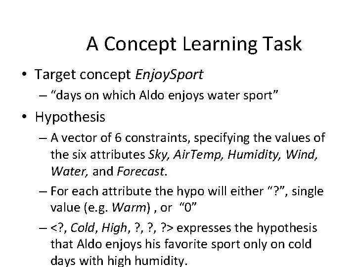
A Concept Learning Task • Target concept Enjoy. Sport – “days on which Aldo enjoys water sport” • Hypothesis – A vector of 6 constraints, specifying the values of the six attributes Sky, Air. Temp, Humidity, Wind, Water, and Forecast. – For each attribute the hypo will either “? ”, single value (e. g. Warm) , or “ 0” – <? , Cold, High, ? , ? > expresses the hypothesis that Aldo enjoys his favorite sport only on cold days with high humidity.

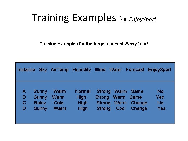
Training Examples for Enjoy. Sport Training examples for the target concept Enjoy. Sport Instance Sky Air. Temp Humidity Wind Water Forecast Enjoy. Sport A B C D Sunny Rainy Sunny Warm Cold Warm Normal High Strong Warm Same Strong Warm Change Strong Cool Change No Yes

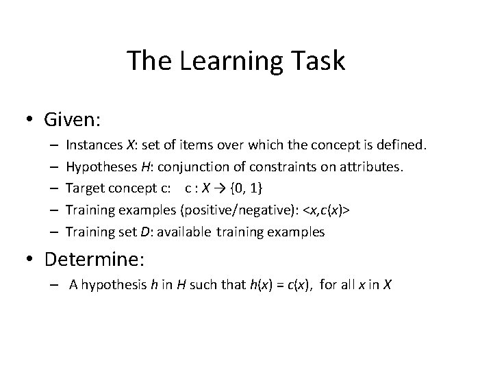
The Learning Task • Given: – – – Instances X: set of items over which the concept is defined. Hypotheses H: conjunction of constraints on attributes. Target concept c: c : X → {0, 1} Training examples (positive/negative): <x, c(x)> Training set D: available training examples • Determine: – A hypothesis h in H such that h(x) = c(x), for all x in X

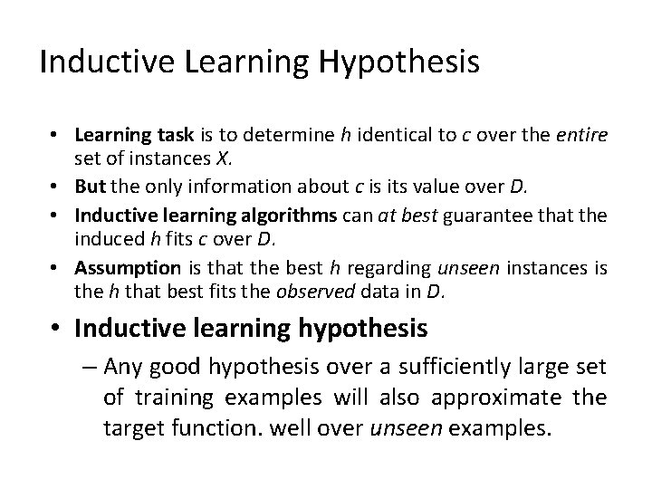
Inductive Learning Hypothesis • Learning task is to determine h identical to c over the entire set of instances X. • But the only information about c is its value over D. • Inductive learning algorithms can at best guarantee that the induced h fits c over D. • Assumption is that the best h regarding unseen instances is the h that best fits the observed data in D. • Inductive learning hypothesis – Any good hypothesis over a sufficiently large set of training examples will also approximate the target function. well over unseen examples.

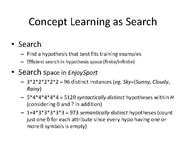
Concept Learning as Search • Search – Find a hypothesis that best fits training examples – Efficient search in hypothesis space (finite/infinite) • Search space in Enjoy. Sport – 3*2*2*2 = 96 distinct instances (eg. Sky={Sunny, Cloudy, Rainy} – 5*4*4*4 = 5120 syntactically distinct hypotheses within H (considering 0 and ? in addition) – 1+4*3*3*3 = 973 semantically distinct hypotheses (count just one 0 for each attribute since every hypo having one or more 0 symbols is empty)

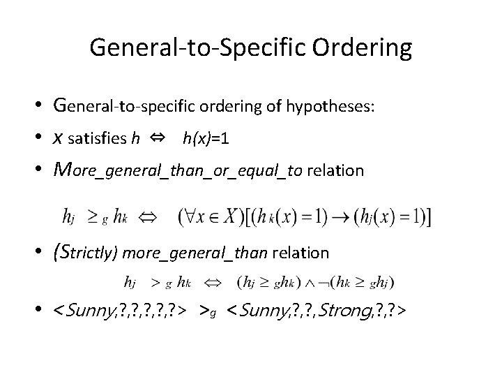
General-to-Specific Ordering • General-to-specific ordering of hypotheses: • x satisfies h ⇔ h(x)=1 • More_general_than_or_equal_to relation • (Strictly) more_general_than relation • <Sunny, ? , ? , ? > >g <Sunny, ? , Strong, ? >

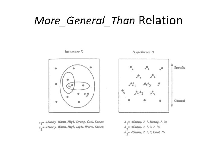
More_General_Than Relation

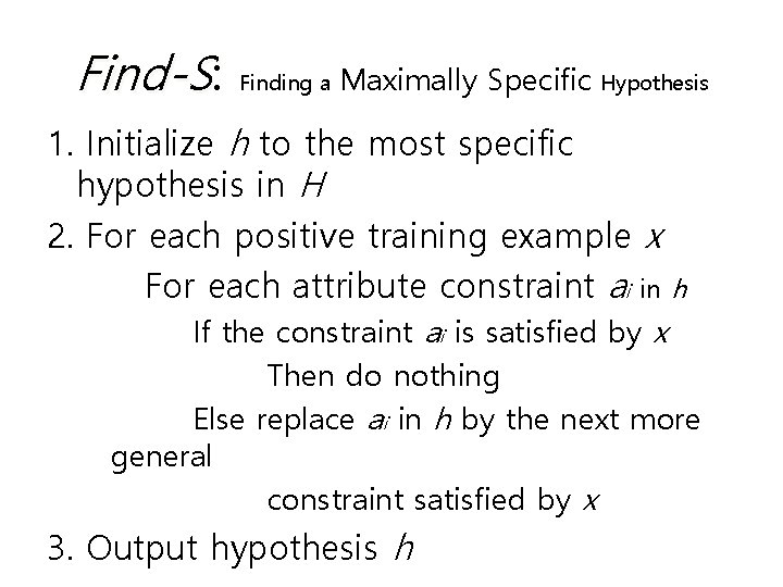
Find-S: Finding a Maximally Specific Hypothesis 1. Initialize h to the most specific hypothesis in H 2. For each positive training example x For each attribute constraint ai in h If the constraint ai is satisfied by x Then do nothing Else replace ai in h by the next more general constraint satisfied by x 3. Output hypothesis h

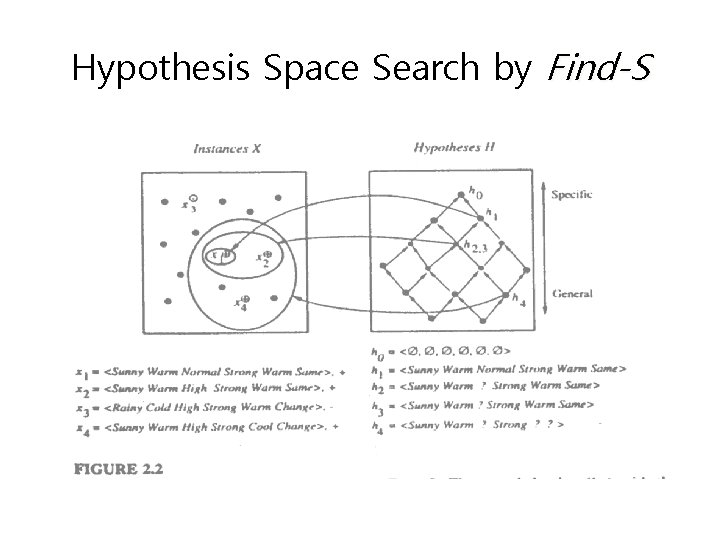
Hypothesis Space Search by Find-S

Properties of Find-S • Ignores every negative example (no revision to h required in response to negative examples). Why? What’re the assumptions for this? • Guaranteed to output the most specific hypothesis consistent with the positive training examples (for conjunctive hypothesis space). • Final h also consistent with negative examples provided the target c is in H and no error in D.

Weaknesses of Find-S • Has the learner converged to the correct target concept? No way to know whether the solution is unique. • Why prefer the most specific hypothesis? How about the most general hypothesis? • Are the training examples consistent? Training sets containing errors or noise can severely mislead the algorithm Find-S. • What if there are several maximally specific consistent hypotheses? No backtrack to explore a different branch of partial ordering.

Version Spaces (VSs) • Output all hypotheses consistent with the training examples. • Version space – Consistent(h, D) ⇔ (∀<x, c(x)> D) h(x) = c(x) – VSH, D ⇔ {h H | Consistent(h, D)} • List-Then-Eliminate Algorithm – Lists all hypotheses, then removes inconsistent ones. – Applicable to finite H

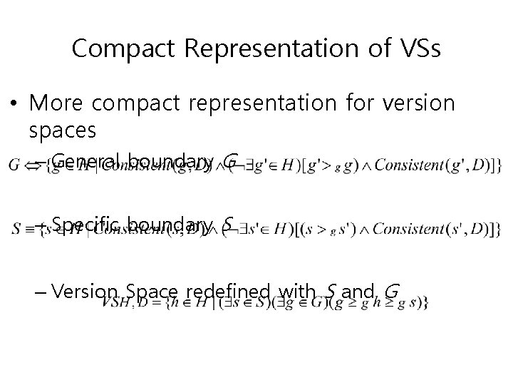
Compact Representation of VSs • More compact representation for version spaces – General boundary G – Specific boundary S – Version Space redefined with S and G

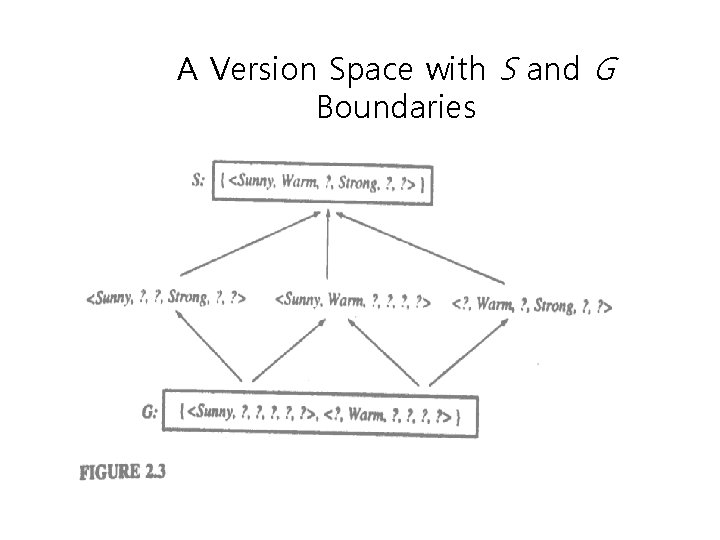
A Version Space with S and G Boundaries

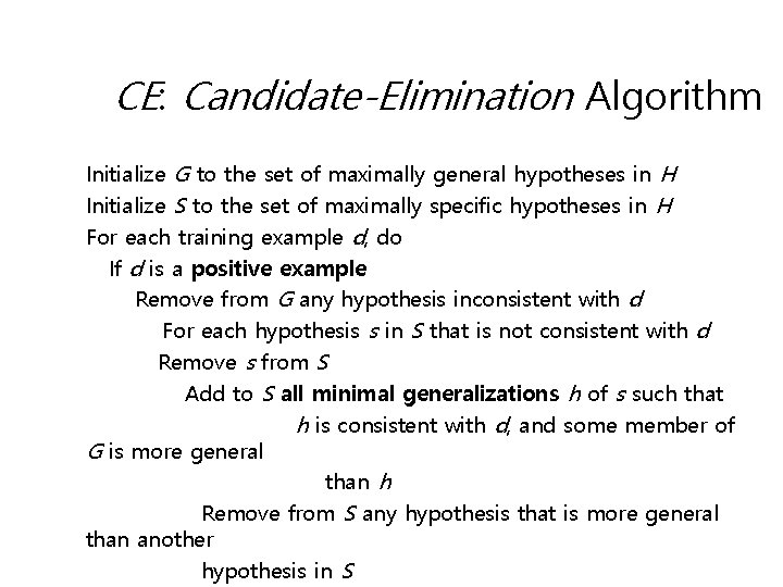
CE: Candidate-Elimination Algorithm Initialize G to the set of maximally general hypotheses in H Initialize S to the set of maximally specific hypotheses in H For each training example d, do If d is a positive example Remove from G any hypothesis inconsistent with d For each hypothesis s in S that is not consistent with d Remove s from S Add to S all minimal generalizations h of s such that h is consistent with d, and some member of G is more general than h Remove from S any hypothesis that is more general than another hypothesis in S

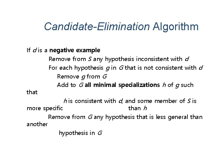
Candidate-Elimination Algorithm If d is a negative example Remove from S any hypothesis inconsistent with d For each hypothesis g in G that is not consistent with d Remove g from G Add to G all minimal specializations h of g such that h is consistent with d, and some member of S is more specific than h Remove from G any hypothesis that is less general than another hypothesis in G

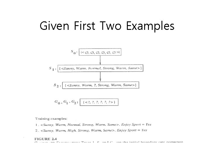
Given First Two Examples

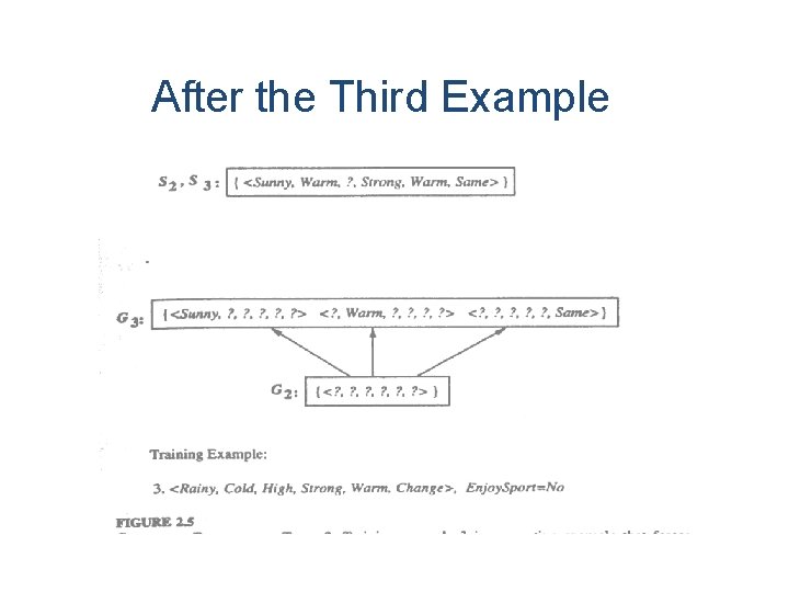
After the Third Example

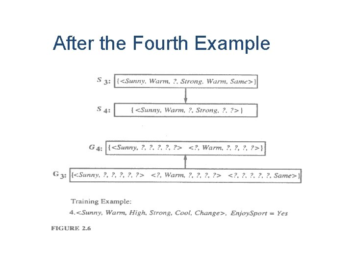
After the Fourth Example

Training Sample 1 & 2 are Positive examples so it forces the S boundary of the Version Space to become increasingly general. Training Sample 3 is a negative examples. In this –ve example reveals that the G boundary of the version space is overly general. Therefore the H in G predicts incorrectly as positive rather than –ve. The H in G boundary must be specialized untill it correctly classifies –ve.

There are several alternates for minimally more specific hypothesis. The –ve example that forces the G 2 to be specialized to G 3. The hypothesis h=<? , normal, ? , ? > is a minimal specialization of G 2 that labels the new example as –ve, but it is not included in G 3 due to inconsistent. After these 4 examples, S 4 and G 4 delimit the version space of all hypothesis consistent with the set of increasingly observed training examples. The entire version space including those hypothesis bounded by S 4 and G 4. this learned version space is independent of the square in which the training examples are presented.

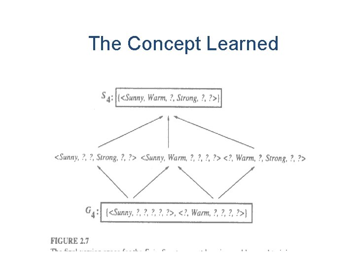
The Concept Learned

Remarks on Candidate Elimination • Will the CE algorithm converge to the correct hypothesis? When target function is true. • What training example should the learner request next? Learner may conduct experiments or consult a teacher. • How can partially learned concepts be used? It is possible to classify certain example with the same degree of confidence as if the target concept had been uniquely identified.

When Does CE Converge? • Will the Candidate-Elimination algorithm converge to the correct hypothesis? • Prerequisites 1. No error in training examples 2. The target hypothesis exists which correctly describes c(x). • If S and G boundary sets converge to an empty set, this means there is no hypothesis in H consistent with observed

Fundamental Questions for Inductive Inference • CE will converge toward the target concept provided that it is contained in its initial hypo space and training examples contain no errors. • What if the target concept is not contained in the hypo space? • One solution: Use a hypothesis space that includes every possible hypothesis (more expressive hypo space). • New problem: Generalize poorly or do not generalize at all.

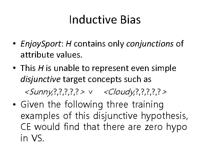
Inductive Bias • Enjoy. Sport: H contains only conjunctions of attribute values. • This H is unable to represent even simple disjunctive target concepts such as <Sunny, ? , ? , ? > ∨ <Cloudy, ? , ? , ? > • Given the following three training examples of this disjunctive hypothesis, CE would find that there are zero hypo in VS.

• Biased Hypothesis Space • Un-Biased Hypothesis Learning • Futility of Bias-Free Learning

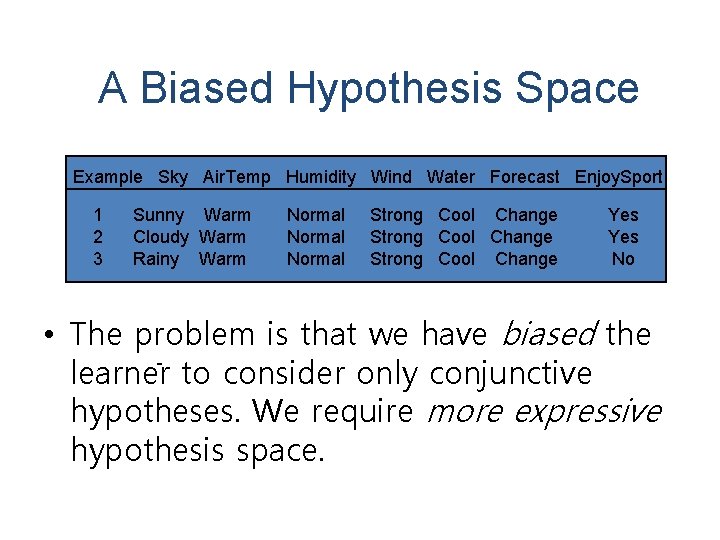
A Biased Hypothesis Space Example Sky Air. Temp Humidity Wind Water Forecast Enjoy. Sport 1 2 3 Sunny Warm Cloudy Warm Rainy Warm Normal Strong Cool Change Yes No • The problem is that we have biased the learner- to consider only conjunctive hypotheses. We require more expressive hypothesis space.

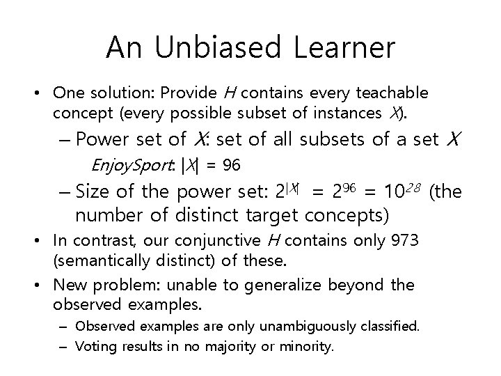
An Unbiased Learner • One solution: Provide H contains every teachable concept (every possible subset of instances X). – Power set of X: set of all subsets of a set X Enjoy. Sport: |X| = 96 – Size of the power set: 2|X| = 296 = 1028 (the number of distinct target concepts) • In contrast, our conjunctive H contains only 973 (semantically distinct) of these. • New problem: unable to generalize beyond the observed examples. – Observed examples are only unambiguously classified. – Voting results in no majority or minority.

Futility of Bias-Free Learning • Fundamental property of inductive inference: “A learner that makes no a priori assumptions regarding the identity of the target concept has no rational basis for classifying any unseen instances. ”

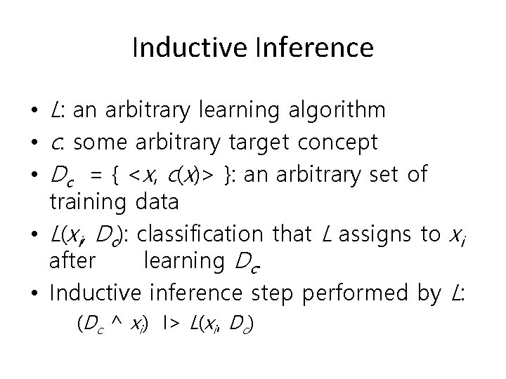
Inductive Inference • L: an arbitrary learning algorithm • c: some arbitrary target concept • Dc = { <x, c(x)> }: an arbitrary set of training data • L(xi, Dc): classification that L assigns to xi after learning Dc. • Inductive inference step performed by L: (Dc ^ xi) I> L(xi, Dc)

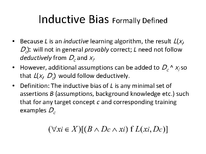
Inductive Bias Formally Defined • Because L is an inductive learning algorithm, the result L(xi, Dc): will not in general provably correct; L need not follow deductively from Dc and xi. • However, additional assumptions can be added to Dc ^ xi so that L(xi, Dc) would follow deductively. • Definition: The inductive bias of L is any minimal set of assertions B (assumptions, background knowledge etc. ) such that for any target concept c and corresponding training examples Dc

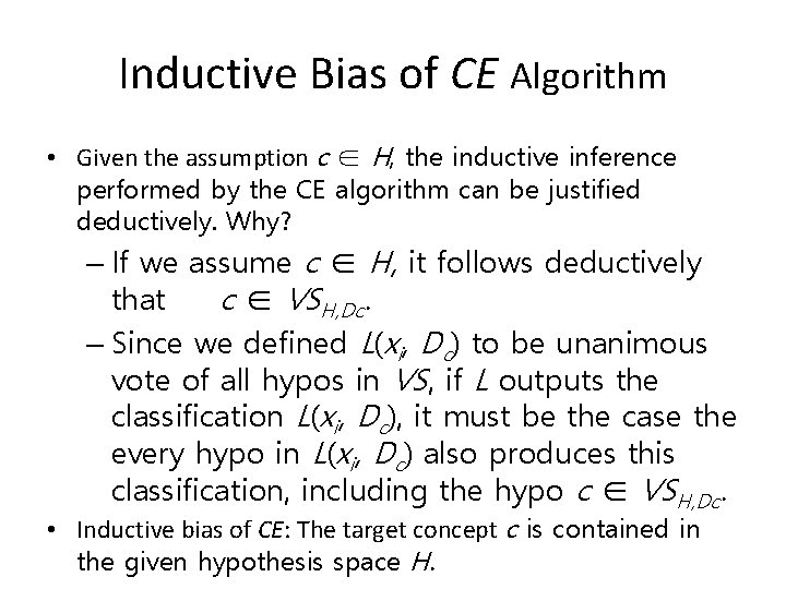
Inductive Bias of CE Algorithm • Given the assumption c ∈ H, the inductive inference performed by the CE algorithm can be justified deductively. Why? – If we assume c ∈ H, it follows deductively that c ∈ VSH, Dc. – Since we defined L(xi, Dc) to be unanimous vote of all hypos in VS, if L outputs the classification L(xi, Dc), it must be the case the every hypo in L(xi, Dc) also produces this classification, including the hypo c ∈ VSH, Dc. • Inductive bias of CE: The target concept c is contained in the given hypothesis space H.

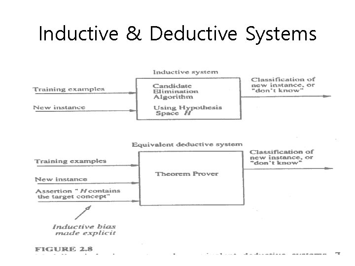
Inductive & Deductive Systems

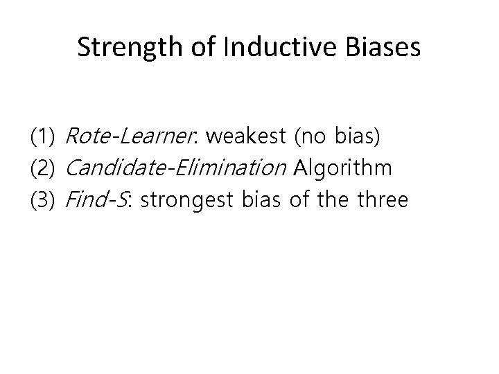
Strength of Inductive Biases (1) Rote-Learner: weakest (no bias) (2) Candidate-Elimination Algorithm (3) Find-S: strongest bias of the three

Inductive Bias of Rote-Learner • Simply stores each observed training example in memory. • New instances are classified by looking them up in memory: – If it is found in memory, the stored classification is returned. – Otherwise, the system refuses to classify the new instance. • No inductive bias: The classifications for new instances follow deductively from D with no additional assumptions required.

Inductive Bias of Cand. -Ellim. • New instances are classified only if all hypos in VS agree. Otherwise, it refuses to classify. • Inductive bias: The target concept can be represented in its hypothesis space. • This inductive bias is stronger than that of rote-learner since CE will classify some instances that the rote-learner will not.

Inductive Bias of Find-S • Find the most specific hypo consistent with D and uses this hypo to classify new instances. • Even stronger inductive biase – The target concept can be described in its hypo space. – All instances are negative unless opposite is entailed by its other knowledge (default reasoning)

Summary (1/3) • Concept learning can be cast as a problem of searching through a large predefined space of potential hypotheses. • General-to-specific partial ordering of hypotheses provides a useful structure for search. • Find-S algorithm performs specific-togeneral search to find the most specific hypothesis.

Summary (2/3) • Candidate-Elimination algorithm computes version space by incrementally computing the sets of maximally specific (S) and maximally general (G) hypotheses. • S and G delimit the entire set of hypotheses consistent with the data. • Version spaces and Candidate. Elimination algorithm provide a useful conceptual framework for studying

Summary (3/3) • Candidate-Elimination algorithm is not robust to noisy data or to situations where the unknown target concept is not expressible in the provided hypothesis space. • Inductive bias in Candidate-Elimination algorithm is that target concept exists in H • If the hypothesis space is enriched to the point where there is every possible hypothesis (the power set of instances), then this will remove the inductive bias of CE and thus remove the ability to classify any instance beyond the observed examples.

Web Links • https: //www. youtube. com/watch? v=w 1 vu. Qthc. Xs&list=PLyq. Sp. Qz. TE 6 M-SISTun. GRBRi. Zk 7 op. YBf_K&index=2 • https: //www. youtube. com/watch? v=wh. SKA 8 a. O 6 x. Q&list=PLyq. Sp Qz. TE 6 M-SISTun. GRBRi. Zk 7 op. YBf_K&index=3 • https: //www. youtube. com/watch? v=EWm. Ck. Vf. Pn. J 8&list=PL 3 p. Gy 4 Htqw. D 2 a 57 wl 7 Cl 7 tmfxfk 7 JWJ 9 Y&index=3 • https: //www. youtube. com/watch? v=9 v. Mp. Hk 44 XXo&list=PL 1 x. HD 4 vte. KYVpa. Iiy 295 pg 6_SY 5 qznc 77&index=5 • https: //www. youtube. com/watch? v=E 3 l 26 b. Tdtx. I&list=PL 3 p. Gy 4 H tqw. D 2 a 57 wl 7 Cl 7 tmfxfk 7 JWJ 9 Y&index=19 • These NPTEL videos lectures are useful to get the basic of machine learning, artificial intelligence, and their algorithms how it can be used for the real world problems is been covered in these videos.