MODIS and VIIRS Geolocation Error and Longterm Trend

MODIS and VIIRS Geolocation Error and Long-term Trend Analysis with Automated Correction Techniques using Kalman Filtering Masahiro Nishihama Sigma Space Corporation Lanham, Maryland, USA (20706) mash. nishihama@nasa. gov Robert E. Wolfe NASA Goddard Space Flight Center, Code 614. 5 Greenbelt, Maryland, USA (20771) robert. e. wolfe@nasa. gov IGARSS 2011 July 24 -29, Vancouver Canada

INTRODUCTION - Accurate geolocation of remote sensing data is needed for Earth science research and applications - Initial on-orbit bias removal is performed immediately after launch - Analysis and removal of long-term geolocation bias is needed to maintain accurate geolocation throughout multi-year missions - Analysis and removal of the within-orbit trend is also needed because of thermal effects on instrument pointing - Current approach is a manual least-squares analysis that uses linear and sinusoidal curves to remove both the long-term and within-orbit trends - This presentation discusses two Kalman filtering approaches that are being considered to replace the current manual least-squares approach - These new techniques can be applied to the Moderate-Resolution Imaging Spectroradiometer (MODIS) instruments and the future Visible Infrared Imaging Radiometer Suite (VIIRS) instrument. IGARSS’ 11 -Nishihama et al. 2

Background • MODIS - Launched on NASA’s Earth Observing System (EOS) Terra spacecraft in December 1999, and started collecting data in February 2000 - MODIS on Aqua spacecraft in May 2002, began collecting data in July 2002 - whisk-broom sensor with 36 spectral bands; 2 at 250 m, 5 at 500 m and 29 at 1 km nadir spatial resolution - “Ideal” band is located at the center of focal planes (1 km resolution) • Geolocation Components 1) sensor geometry 3) ECI and ECR IGARSS’ 11 -Nishihama et al. 2) spacecraft orbit-attitude relationship 4) Earth – Terrain height 3

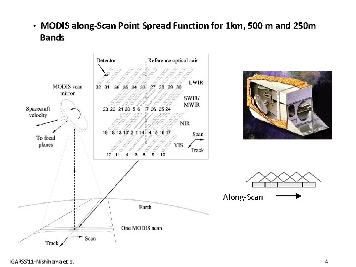
• MODIS along-Scan Point Spread Function for 1 km, 500 m and 250 m Bands Along-Scan IGARSS’ 11 -Nishihama et al. 4

• Geolocation Error Analysis Tools - Use of Control Point Chip Library 1200 TM Landsat subscenes ( Red band Band 3) - Estimation of Geolocation Residuals and Management using Band 1 (250 m) - Red band - Parameter (roll/pitch/yaw error ) Estimation Program 1) Non-linear sensor model for residuals to Linear model, 2) Estimation of roll/pith/yaw from along-track/scan errors - Estimated Initial Geolocation Error 1) Terra Geo Error(March 2000) roll: 243’’ pitch: -354” yaw: 0 2) Aqua Geo Error(July 2002) roll: 424” pitch: -26” yaw: -51” IGARSS’ 11 -Nishihama et al. 5

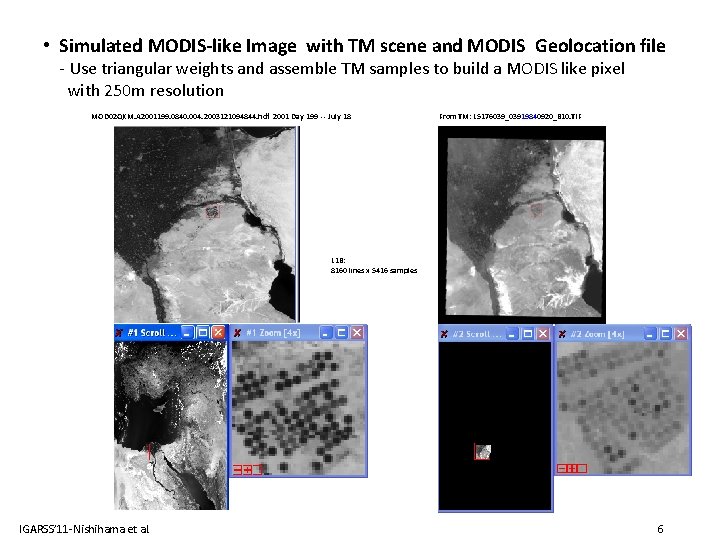
• Simulated MODIS-like Image with TM scene and MODIS Geolocation file - Use triangular weights and assemble TM samples to build a MODIS like pixel with 250 m resolution MOD 02 QKM. A 2001199. 0840. 004. 2003121094844. hdf 2001 Day 199 -- July 18 From TM: L 5176039_03919840920_B 10. TIF L 1 B: 8160 lines x 5416 samples IGARSS’ 11 -Nishihama et al. 6

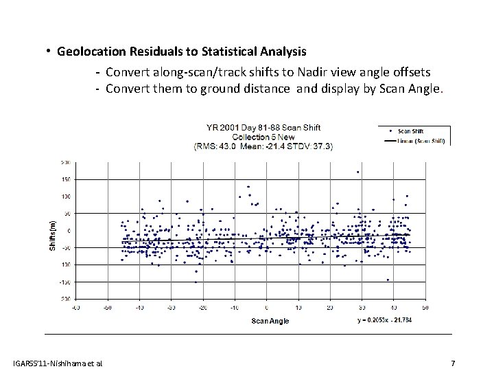
• Geolocation Residuals to Statistical Analysis - Convert along-scan/track shifts to Nadir view angle offsets - Convert them to ground distance and display by Scan Angle. IGARSS’ 11 -Nishihama et al. 7

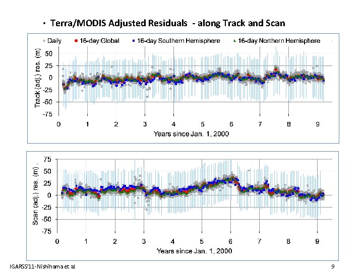
• Long Term Geolocation Error Trend and Analysis - One year or more of accumulated residual records needed - Trend (linear and annual cyclic) with a combination of linear and sinusoidal curve to fit the scan and track directions - Remove additional smaller within-orbit variations caused by temperature variation - Reduced geolocation error to less than 50 m Root Mean Square Error (RMSE) for MODIS/Terra and 60 m RMSE for MODIS/Aqua. Note: Difference in Geolocation Accuracy between Terra and Aqua - Terra orbit is identical to Landsat orbit, - Terra observes a similar Earth shadow as TM does (10: 30 AM) - Motion of AMSR-E Parabolic Reflector 1. 6 meters in diameter on top of Aqua IGARSS’ 11 -Nishihama et al. 8

• Terra/MODIS Adjusted Residuals - along Track and Scan IGARSS’ 11 -Nishihama et al. 9

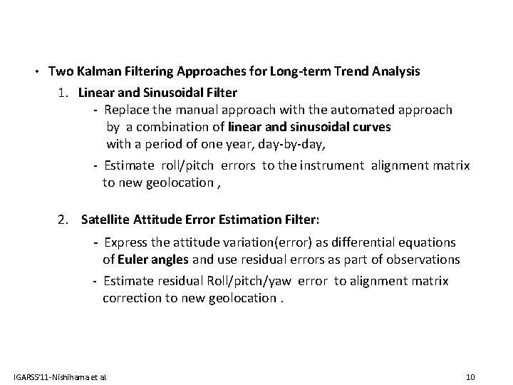
• Two Kalman Filtering Approaches for Long-term Trend Analysis 1. Linear and Sinusoidal Filter - Replace the manual approach with the automated approach by a combination of linear and sinusoidal curves with a period of one year, day-by-day, - Estimate roll/pitch errors to the instrument alignment matrix to new geolocation , 2. Satellite Attitude Error Estimation Filter: - Express the attitude variation(error) as differential equations of Euler angles and use residual errors as part of observations - Estimate residual Roll/pitch/yaw error to alignment matrix correction to new geolocation. IGARSS’ 11 -Nishihama et al. 10

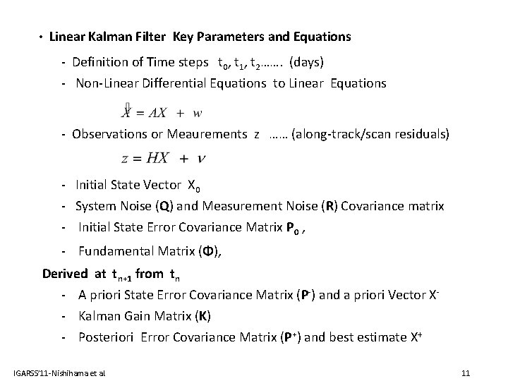
• Linear Kalman Filter Key Parameters and Equations - Definition of Time steps t 0, t 1, t 2……. (days) - Non-Linear Differential Equations to Linear Equations - Observations or Meaurements z …… (along-track/scan residuals) - Initial State Vector X 0 - System Noise (Q) and Measurement Noise (R) Covariance matrix - Initial State Error Covariance Matrix P 0 , - Fundamental Matrix (Φ), Derived at tn+1 from tn - A priori State Error Covariance Matrix (P-) and a priori Vector X- Kalman Gain Matrix (K) - Posteriori Error Covariance Matrix (P+) and best estimate X+ IGARSS’ 11 -Nishihama et al. 11

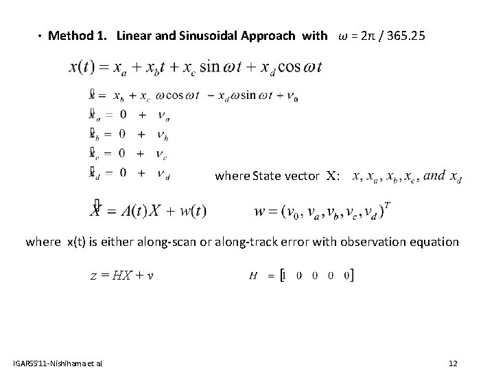
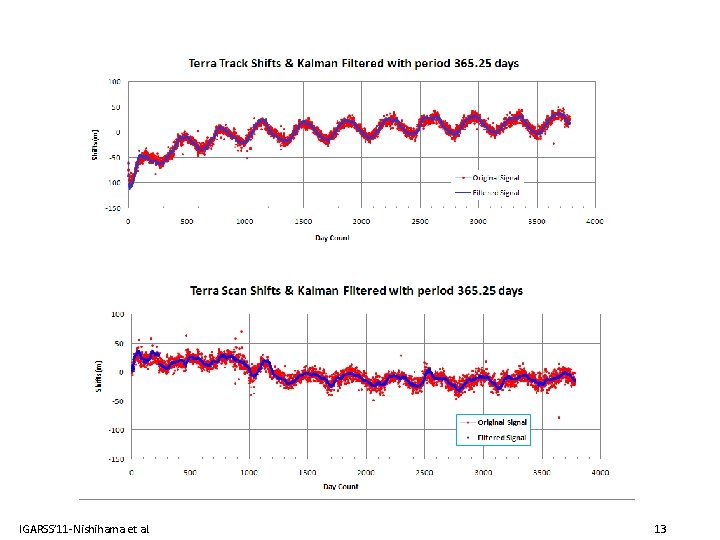
• Method 1. Linear and Sinusoidal Approach with ω = 2π / 365. 25 where State vector X: where x(t) is either along-scan or along-track error with observation equation z = HX + ν IGARSS’ 11 -Nishihama et al. 12

IGARSS’ 11 -Nishihama et al. 13

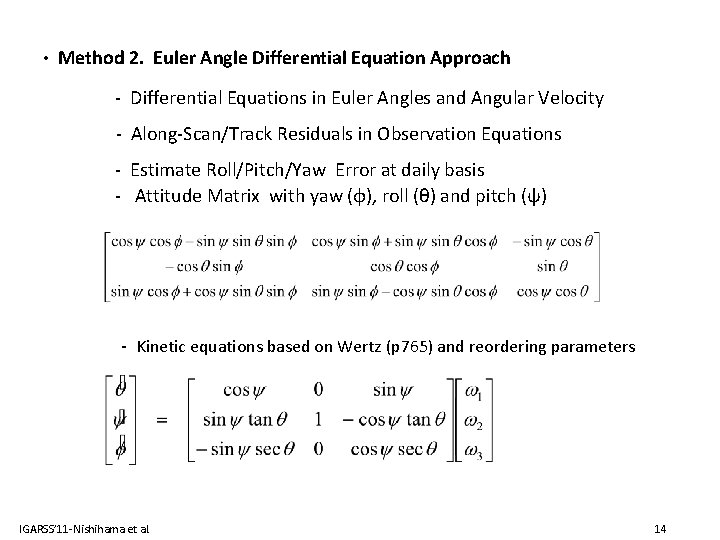
• Method 2. Euler Angle Differential Equation Approach - Differential Equations in Euler Angles and Angular Velocity - Along-Scan/Track Residuals in Observation Equations - Estimate Roll/Pitch/Yaw Error at daily basis - Attitude Matrix with yaw (φ), roll (θ) and pitch (ψ) - Kinetic equations based on Wertz (p 765) and reordering parameters IGARSS’ 11 -Nishihama et al. 14

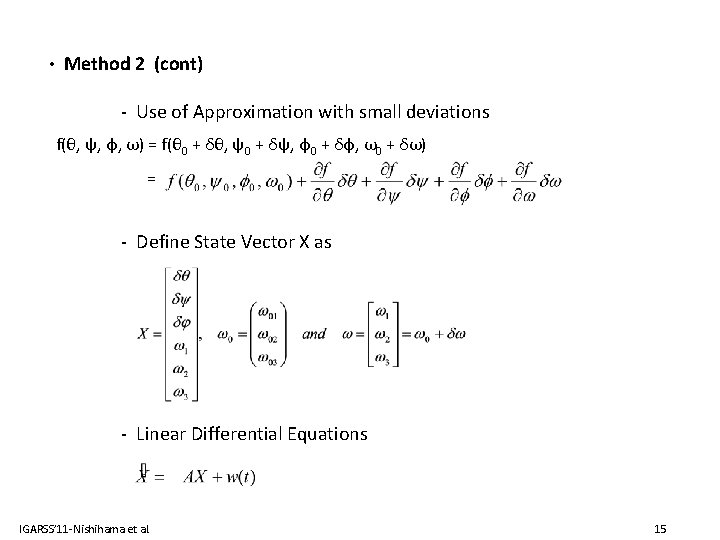
• Method 2 (cont) - Use of Approximation with small deviations f(θ, ψ, φ, ω) = f(θ 0 + δθ, ψ0 + δψ, φ0 + δφ, ω0 + δω) = - Define State Vector X as - Linear Differential Equations IGARSS’ 11 -Nishihama et al. 15

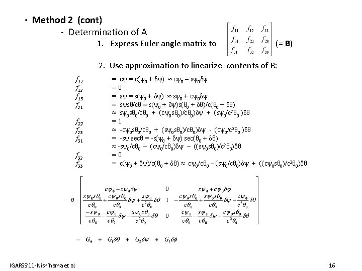
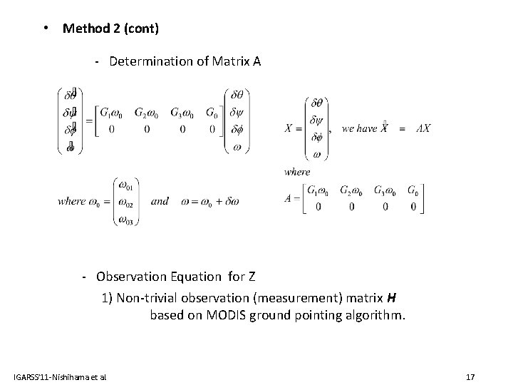
• Method 2 (cont) - Determination of A 1. Express Euler angle matrix to (= B) 2. Use approximation to linearize contents of B: f 11 f 12 f 13 f 21 f 22 f 23 f 31 f 32 f 33 IGARSS’ 11 -Nishihama et al. = cψ = c(ψ0 + δψ) ≈ cψ0 – sψ0δψ =0 = sψ = s(ψ0 + δψ) ≈ sψ0 + cψ0δψ = sψsθ/cθ = s(ψ0 + δψ)s(θ 0 + δθ)/c(θ 0 + δθ) ≈ sψ0 sθ 0/cθ 0 + (cψ0 sθ 0)/cθ 0)δψ + (sψ0/c 2θ 0 )δθ =1 ≈ -cψ0 sθ 0/cθ 0 + (sψ0 sθ 0)/cθ 0)δψ - (cψ0/c 2θ 0 )δθ = -sψ secθ = -s(ψ0 + δψ) sec(θ 0 + δθ) ≈ -sψ0/cθ 0 – (cψ0/cθ 0)δψ – ((sψ0 sθ 0)/c 2θ 0)δθ =0 = c(ψ0 + δψ)/c(θ 0 + δθ) ≈ cψ0/cθ 0 – (sψ0/cθ 0)δψ + ((cψ0 sθ 0)/c 2θ 0)δθ 16

• Method 2 (cont) - Determination of Matrix A - Observation Equation for Z 1) Non-trivial observation (measurement) matrix H based on MODIS ground pointing algorithm. IGARSS’ 11 -Nishihama et al. 17

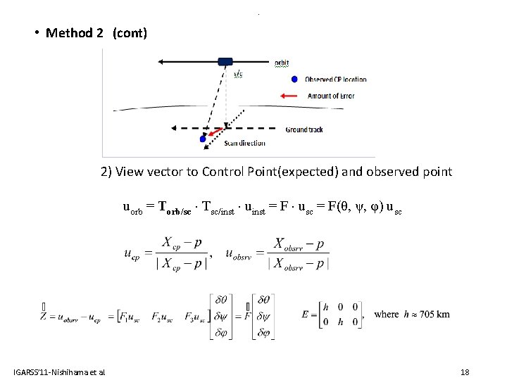
. • Method 2 (cont) 2) View vector to Control Point(expected) and observed point uorb = Torb/sc Tsc/inst uinst = F usc = F(θ, ψ, φ) usc IGARSS’ 11 -Nishihama et al. 18

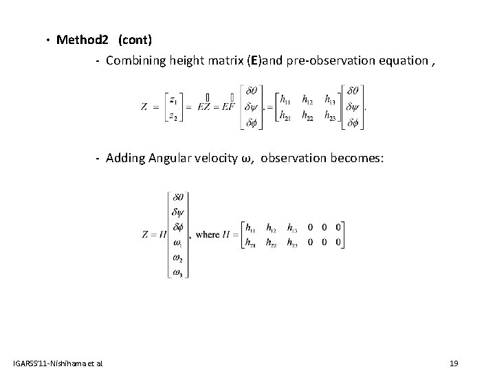
• Method 2 (cont) - Combining height matrix (E)and pre-observation equation , - Adding Angular velocity ω, observation becomes: IGARSS’ 11 -Nishihama et al. 19

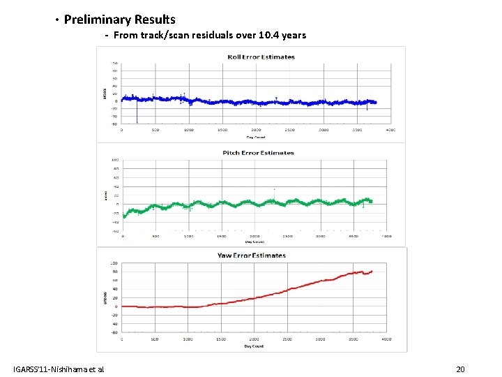
• Preliminary Results - From track/scan residuals over 10. 4 years IGARSS’ 11 -Nishihama et al. 20

DISCUSSION 1. Analysis of both Kalman filtering methods are preliminary, but results of the first method is very promising. 2. The second method needs more tests and examination. Appearance of yaw in the second method is interesting and needs investigation. 3. Further tests will be needed for Aqua data using both methods. 4. Determination of the initial covariance matrices and other parameters is critical, and requires careful attention. 5. The Kalman filters methods are computationally efficient, it took very little time to processing 3800 sample points (~250 ground points are acquired each day). 6. Once fully tested, either of the methods could be implemented, enabling automated daily geolocation parameter updates. IGARSS’ 11 -Nishihama et al. 21