Modern seismometer Three components of motion can be

Modern seismometer

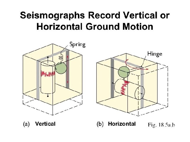
Three components of motion can be measured east-west north-south up-down If you speeded up any earthquake signal and listened to it with a hi fi, it would sound like thunder.

Station 1 Station 2 Station 3 Station 4 Station 5

Different kinds of waves exist within solid materials Body waves – propagate throughout a solid medium

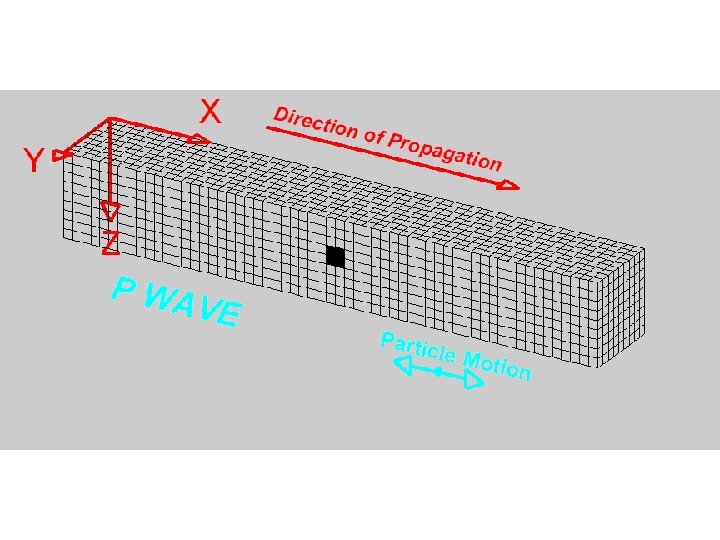
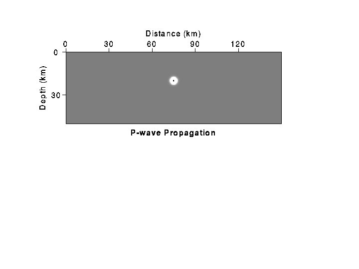
Compressional Waves in one- and twodimensions

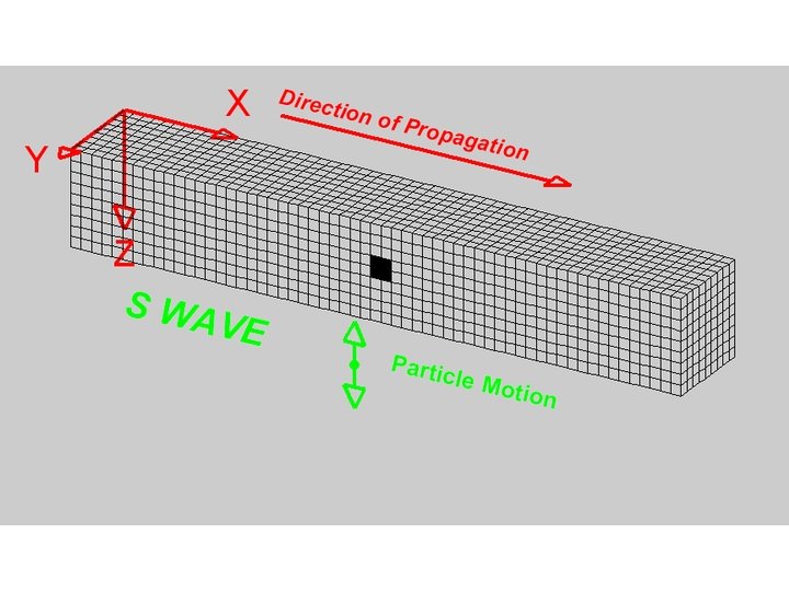
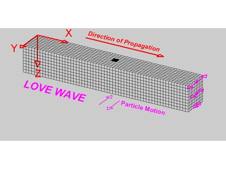
Shear waves in one- and twodimensions

Different types of waves have different speeds Shear velocity (just like waves on a string) Compressional velocity (a bit like a slinky) m= shear modulus = shear stress / shear strain (restoring force to shear) k = bulk modulus = 1/compressibility (restoring force to compression) P-waves travel faster than S-waves (and both travel faster than surface waves)

P-waves get there first…

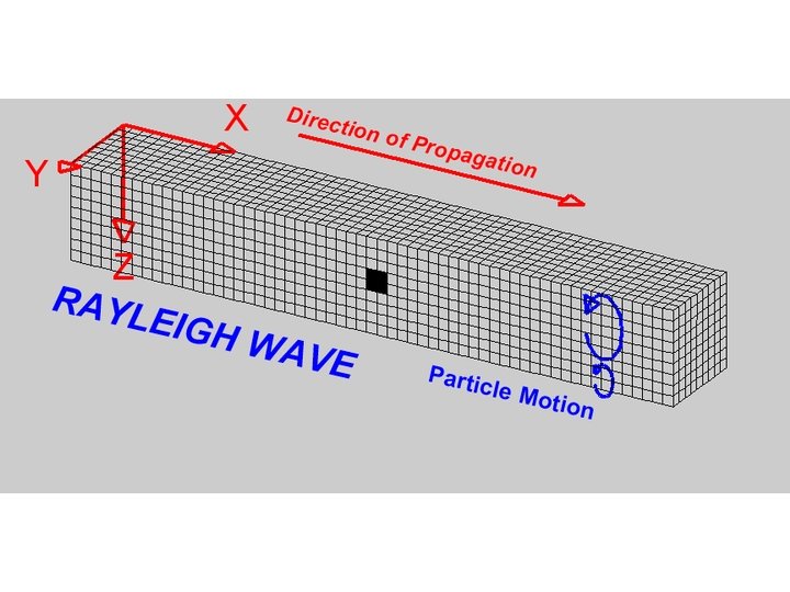
As well as body waves, there are surface waves that propagate along a surface Rayleigh Love

Different kinds of damage…. P-wave Sfc-wave All

P-wave arrival S-wave arrival

Difference between P-wave and S-wave arrival can be used to locate the location of an earthquake more effectively… = Hypocenter

Difference between p- and s-waves can be used to track location

Need 3 stations to isolate location (and the more the better)

The sense of motion can be used to infer the motion that caused it. east-west north-south up-down The “first-motion” of the earthquake signal has information about the motion on the fault that generated it.

The orientation of faults can be determined from seismic networks

Go to board for Snell’s law

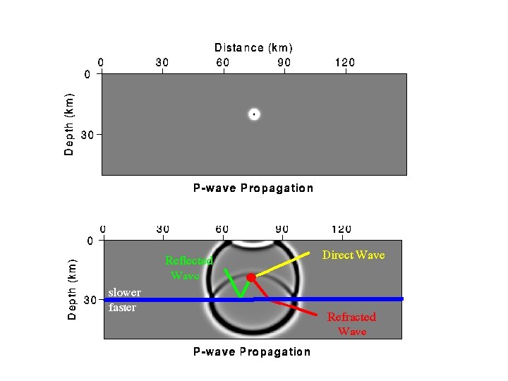
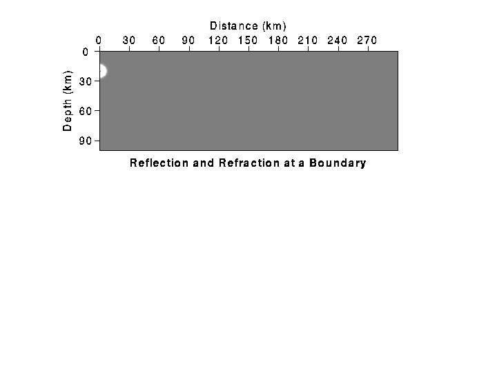
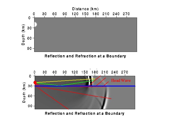
Back to Snell’s Law Any change in wave speed due to composition change with height will cause refraction of rays…. SLOW FAST This one applies to the crust FAST SLOW

Do this on the board

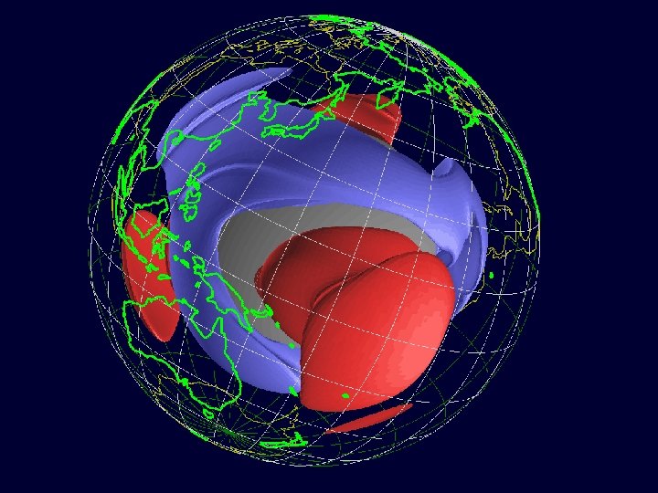
Seismology can be used to infer the structure of the interior of the Earth

$First, recall that wave paths are curved within the Earth due to refraction.$

First, recall that wave paths are curved within the Earth due to refraction.

If the Earth were homogenous in composition…

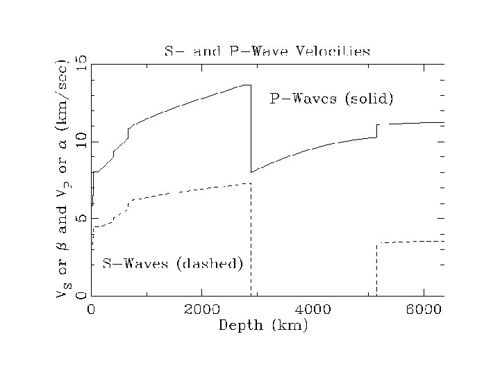
But seismic velocities show great variety of structure moho crust aesthenosphere mesosphere core

S waves cannot propagate through the core, leading to a huge shadow zone S waves cannot propagate in a fluid (fluids cannot support shear stresses)

Shadow zones for P-waves exist but less b/c propagation through the core

Animation of P wave rays

Animation of P wave fronts

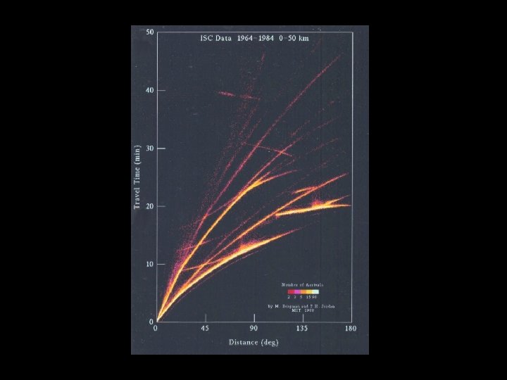
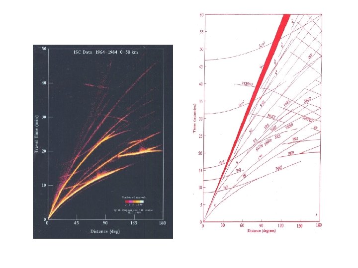
The pathways from any given source are constrained…

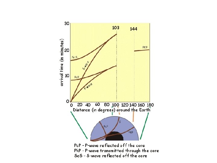
Seismic “phases” are named according to their paths P – P wave only in the mantle PP – P wave reflected off earths surface so there are two P wave segments in the mantle p. P – P wave that travels upward from a deep earthquake, reflects off the surface and then has a single segment in the mantle PKP – P wave that has two segments in the mantle separated by a segment in the core

Ray path examples…

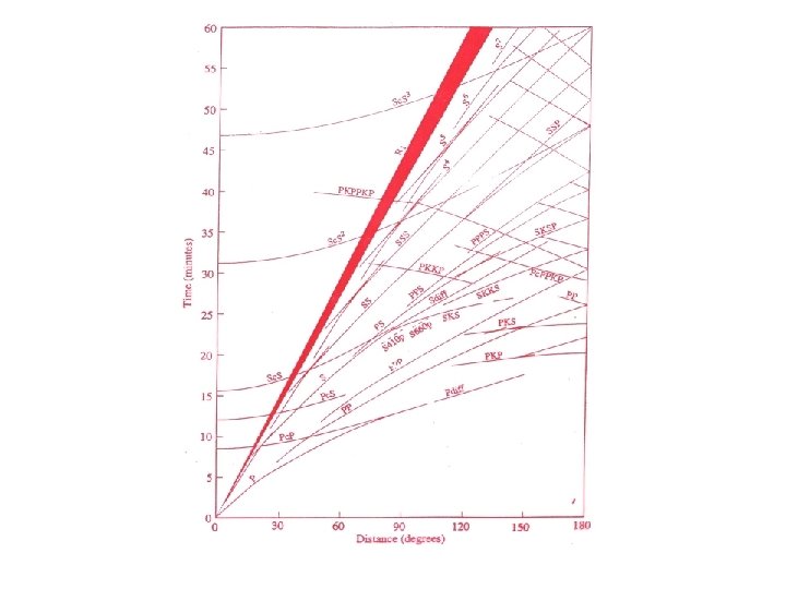
Can be identified from individual seismograms (just about)

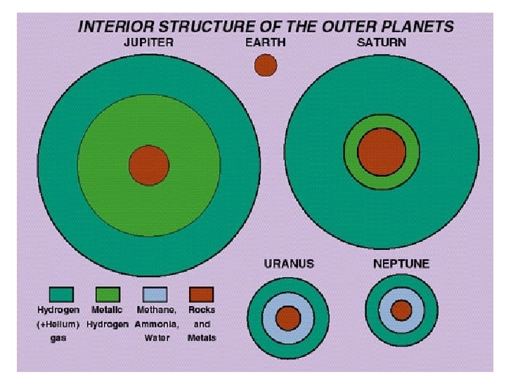
What do we know about the interior composition of the Earth?

How does seismology help?

Velocity beneath Hawaii…

Beneath subduction zones Note the occurrence of deep earthquakes co-located with the down-going slab

Beneath subduction zones

Earthquake number by Richter Scale – variations over time?

Earthquakes are bad for you….

Earthquakes are dangerous Bam, Iran, 2003

Earthquakes are dangerous Chi-chi Taiwan, 1999

Earthquakes are dangerous Olympia, 1965 Seattle, 2001

Earthquakes are dangerous Sichuan, China, 2008

“Helicorder” record of the Sumatra Earthquake and aftershocks recorded in the Czech Republic (December 26, 2004)

Earthquakes are dangerous �El Salvador, 2

Earthquakes are dangerous Kasmir, 2006

Where, when, and how?

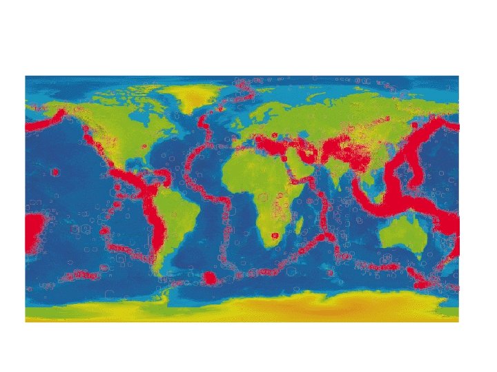
360, 000 earthquakes

Black = 0 to 70; green = 70 -500 km; red = 500 to 700 km

Earthquakes occur across the US U. S. Earthquakes, 1973 -2002 Source, USGS. 28, 332 events. Purple dots are earthquakes below 50 km, the green dot is below 100 km.

Earthquakes in California – different frequency in different sections of the fault 1906 break creeping 1857 break

USGS shake maps – 2% likelihood of seeing peak ground acceleration equal to given color in the next 50 years Units of “g”

USGS shake maps – 2% likelihood of seeing peak ground acceleration equal to given color in the next 50 years Close to home…

USGS shake maps – 10% likelihood of seeing this level of acceleration in The next 50 years

USGS shake maps – Shaking depends on what you’re sitting on.

Different ways of measuring Earthquakes – Part 1. By damage

Different ways of measuring Earthquakes – Part 1. By damage 1966 Parkfield Earthquake Notorious for busted forecast of earthquake frequency.

Different ways of measuring Earthquakes – Part 1. By damage Loma-Prieta Earthquake 1989 I-80 Freeway collapse (65 deaths)

Different ways of measuring Earthquakes – Part 1. By damage Northridge Earthquake, 1994 -January 17, 1994 at 4: 31 AM -the ground acceleration was one of the highest ever instrumentally recorded in an urban area in North America. -72 deaths, 9000 injuries, $20 billion

Different ways of measuring Earthquakes – Part 1. By damage 1906 San Francisco vs. 1811 New Madrid

Different ways of measuring Earthquakes – Part 1. By damage Charleston, MO Earthquake Extent of damage varies widely

Different ways of measuring Earthquakes – Part 2. Richter Scale • quantifies the amount of seismic energy released by an earthquake. • base-10 logarithmic based on the largest displacement, A, from zero on a Wood–Anderson torsion seismometer output. ML = log 10 A − log 10 A 0(DL) A 0 is an empirical function depending only on the distance of the station from the epicenter, DL. • So an earthquake that measures 5. 0 on the Richter scale has a shaking amplitude 10 times larger than one that measures 4. 0. • The effective limit of measurement for local magnitude is about ML = 6. 8 (before seismometer breaks).

Wood Anderson seismometer Uses inertia of copper ball to record accelerations on photo-sensitive paper Wood Anderson seismometer Milne seismometer

Different ways of measuring Earthquakes – Part 2. Richter Scale Two pieces of information used to calculate size of Earthquake: a) Deflection of seismometer, b) distance from source (based on P & S wave arrivals)

Different ways of measuring Earthquakes – Part 2. Richter Scale Equivalency between magnitude and energy

Different ways of measuring Earthquakes – Part 2. Richter Scale

Different ways of measuring Earthquakes – Part 3. By energy released a. Total energy released in an earthquake Earthquake “moment” = force/unit area · displacement · fault area = shear modulus · displacement · fault area = total elastic energy released b. Only a small fraction released as seismic waves Eseismic = M 010 -4. 8 = 1. 6 M 0 · 10 -5 c. Create logarithmic scale (akin to the others)… ‘Moment Magnitude’ Empirical formula

Different ways of measuring Earthquakes – Part 3. By energy released

Different ways of measuring Earthquakes – Part 3. By energy released Equivalence of seismic moment and rupture length a) Depends on earthquake size b) Depends on fault type

Different ways of measuring Earthquakes – Part 3. By energy released Distribution of slip for various Earthquakes Axes are distance along fault & depth. Colors are slip in m

Different ways of measuring Earthquakes – Part 3. By energy released

More information can come from analyzing Earthquake If you speeded up any earthquake signal and listened to it with a hi fi, it would sound like thunder. This is the sound of the 2004 Parkfield 6. 0 Earthquake

Amplitude Narrow band filters A spectrum what you get when you listen to a signal through a series of narrow band filters Frequency

Amplitude vs. time for different frequency bands Lower frequencies have larger amplitudes

Theoretical shapes for earthquakes

And the resulting velocity spectrum

But real earthquakes don’t do this Log 10 Moment (dyne-cm) 1/f (for a box car) 1/f 2 (in reality) Log 10 frequency (hz)

Instead there is a ramp-up time… The time series of displacement looks very similar

Which fits much better with the velocity spectrum • The theoretical spectrum for a “box car” velocity function decreases as 1/f. • Observations show a 1/f 2 behavior. • This can be explained as ramping (i. e acceleration) of the velocity at the start and end.

Get lots of useful information from a velocity spectrum… Scaled moment 1/source duration 1/ramp time