Modern Portfolio Theory History of MPT 1952 Horowitz

Modern Portfolio Theory

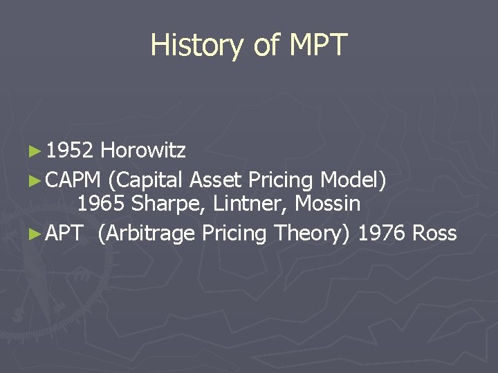
History of MPT ► 1952 Horowitz ► CAPM (Capital Asset Pricing Model) 1965 Sharpe, Lintner, Mossin ► APT (Arbitrage Pricing Theory) 1976 Ross

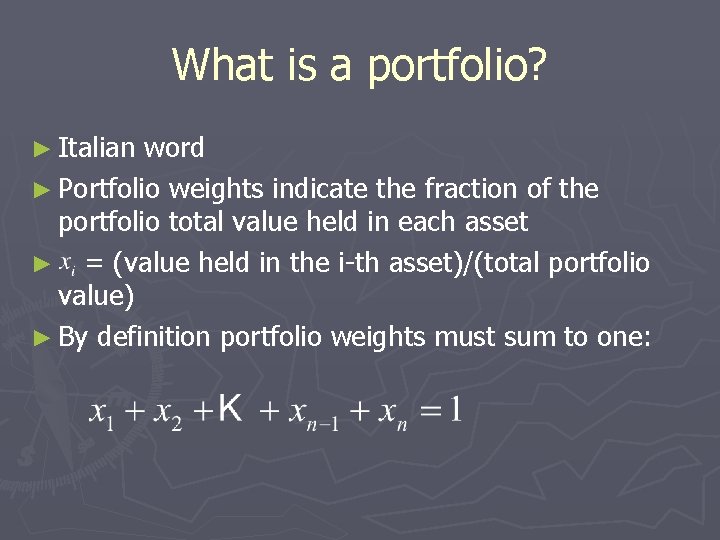
What is a portfolio? ► Italian word ► Portfolio weights indicate the fraction of the portfolio total value held in each asset ► = (value held in the i-th asset)/(total portfolio value) ► By definition portfolio weights must sum to one:

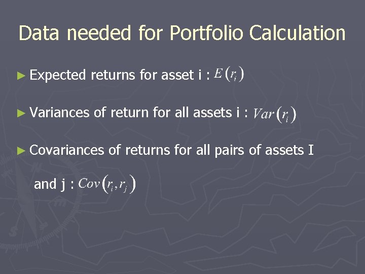
Data needed for Portfolio Calculation ► Expected returns for asset i : ► Variances of return for all assets i : ► Covariances and j : of returns for all pairs of assets I

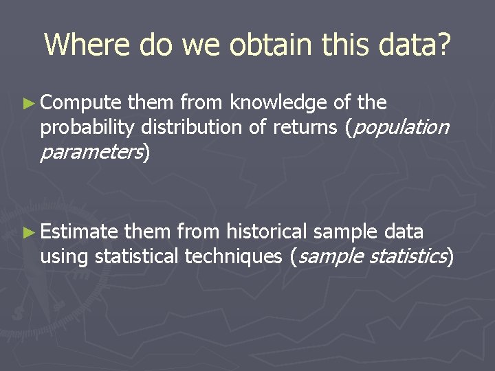
Where do we obtain this data? ► Compute them from knowledge of the probability distribution of returns (population parameters) ► Estimate them from historical sample data using statistical techniques (sample statistics)

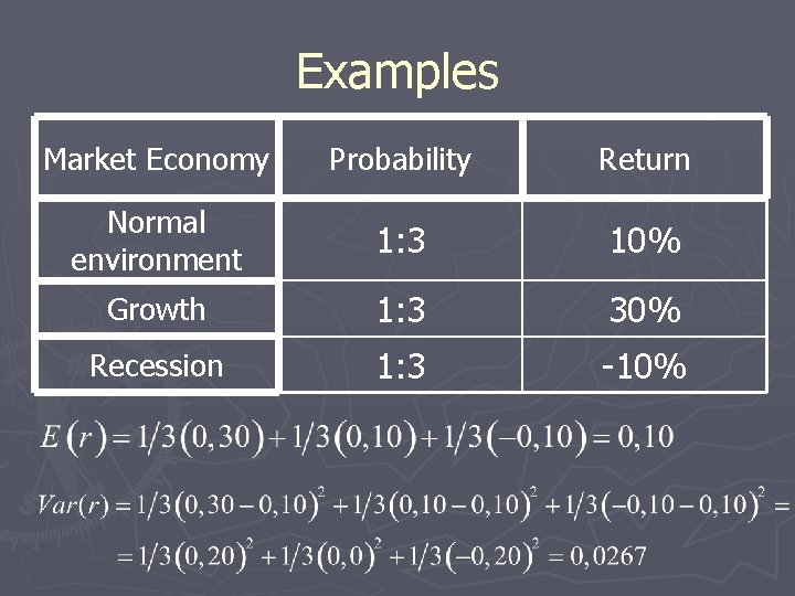
Examples Market Economy Probability Return Normal environment 1: 3 10% Growth 1: 3 30% Recession 1: 3 -10%

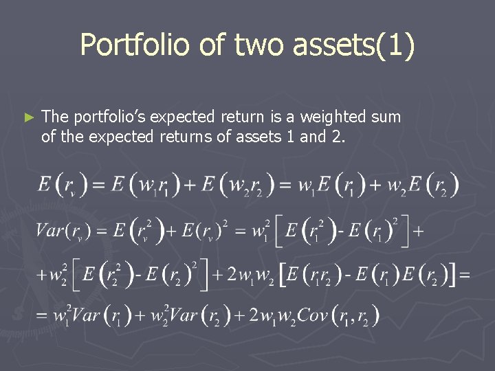
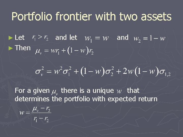
Portfolio of two assets(1) ► The portfolio’s expected return is a weighted sum of the expected returns of assets 1 and 2.

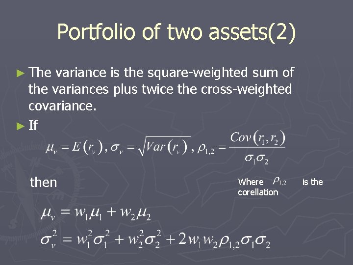
Portfolio of two assets(2) ► The variance is the square-weighted sum of the variances plus twice the cross-weighted covariance. ► If then Where corellation is the

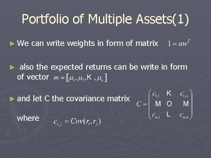
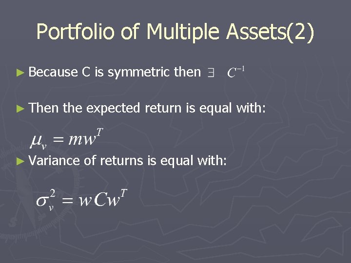
Portfolio of Multiple Assets(1) ► We ► can write weights in form of matrix also the expected returns can be write in form of vector ► and let C the covariance matrix where

Portfolio of Multiple Assets(2) ► Because ► Then C is symmetric then the expected return is equal with: ► Variance of returns is equal with:

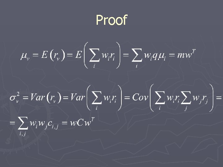
Proof

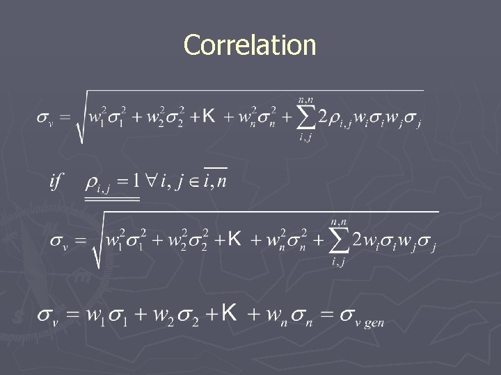
Correlation

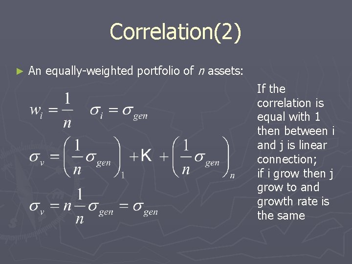
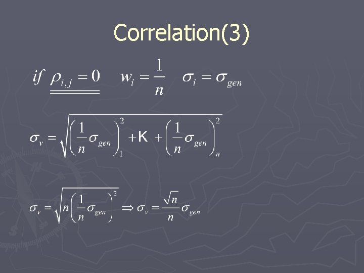
Correlation(2) ► An equally-weighted portfolio of n assets: If the correlation is equal with 1 then between i and j is linear connection; if i grow then j grow to and growth rate is the same

Correlation(3)

Diversification

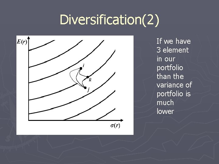
Diversification(2) If we have 3 element in our portfolio than the variance of portfolio is much lower

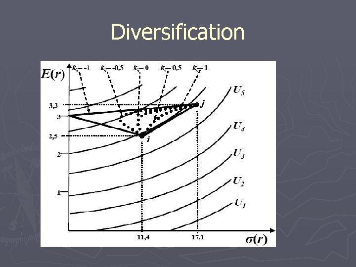
Diversification(3) ► Reducing risk with this technique is called diversification ► Generally the more different the assets are, the greater the diversification. ► The diversification effect is the reduction in portfolio standard deviation, compared with a simple linear combination of the standard deviations, that comes from holding two or more assets in the portfolio ► The size of the diversification effect depends on the degree of correlation

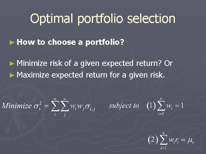
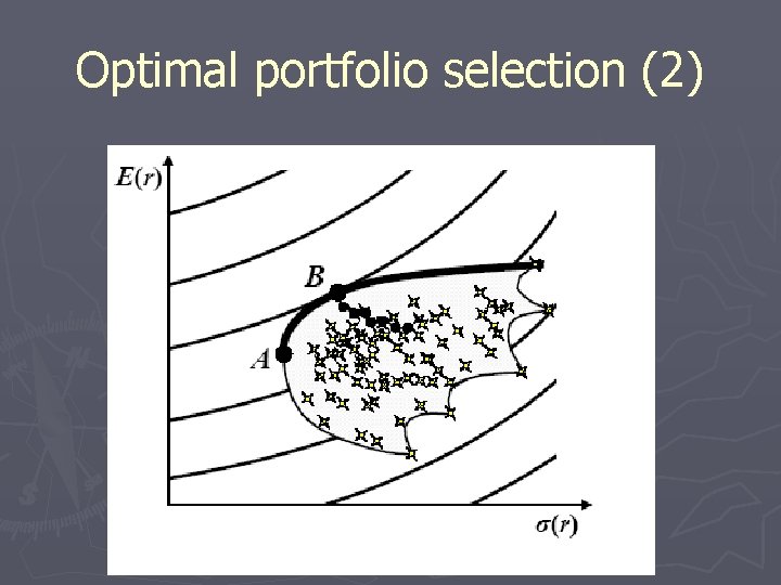
Optimal portfolio selection ► How to choose a portfolio? ► Minimize risk of a given expected return? Or ► Maximize expected return for a given risk.

Optimal portfolio selection (2)

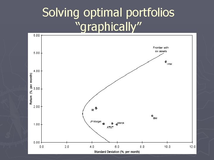
Solving optimal portfolios “graphically”

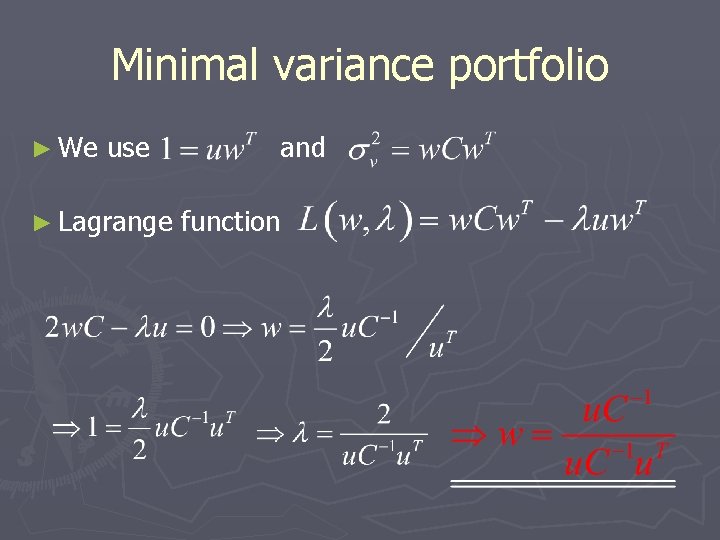
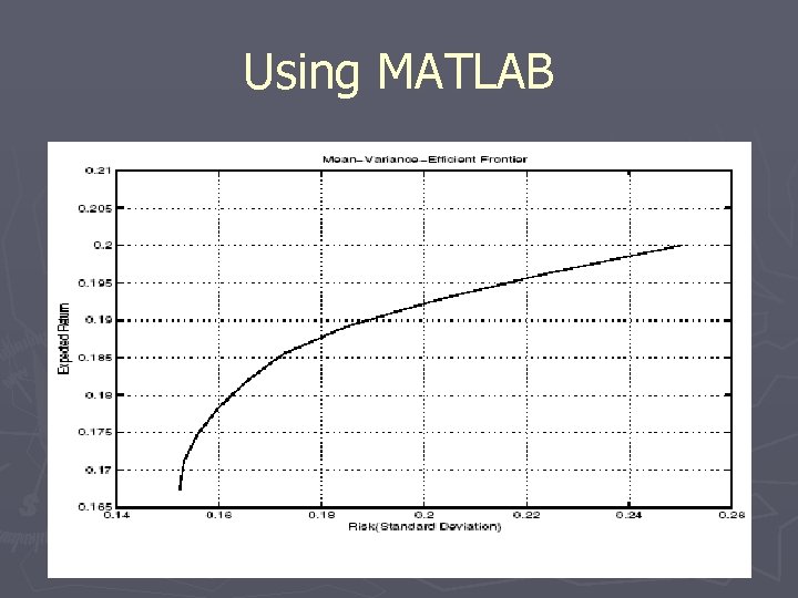
Solving optimal portfolios ► The locus of all frontier portfolios in the plane is called portfolio frontier ► The upper part of the portfolio frontier gives efficient frontier portfolios ► Minimal variance portfolio

Portfolio frontier with two assets ► Let and let and ► Then For a given there is a unique that determines the portfolio with expected return

Minimal variance portfolio ► We use ► Lagrange and function

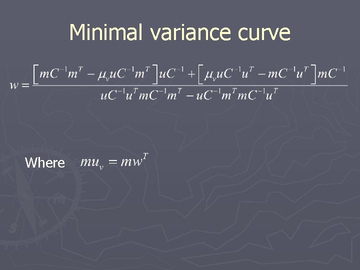
Minimal variance curve Where

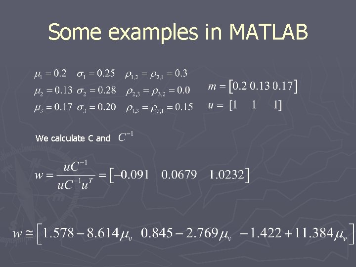
Some examples in MATLAB We calculate C and

Using MATLAB

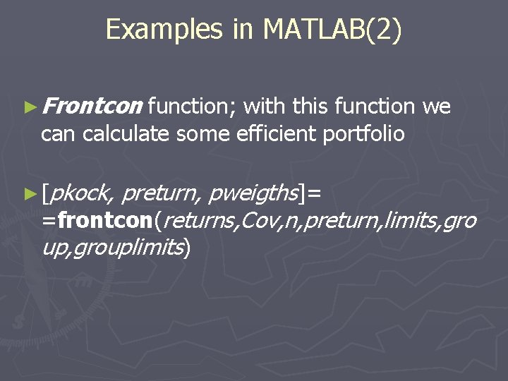
Examples in MATLAB(2) ► Frontcon function; with this function we can calculate some efficient portfolio ► [pkock, preturn, pweigths]= =frontcon(returns, Cov, n, preturn, limits, gro up, grouplimits)

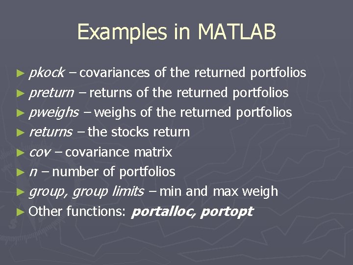
Examples in MATLAB ► pkock – covariances of the returned portfolios ► preturn – returns of the returned portfolios ► pweighs – weighs of the returned portfolios ► returns – the stocks return ► cov – covariance matrix ► n – number of portfolios ► group, group limits – min and max weigh ► Other functions: portalloc, portopt