Models and Algorithms for Complex Networks Theory and

Models and Algorithms for Complex Networks Theory and Algorithms for Link Analysis Ranking, Rank Aggregation, and Voting

Outline § Axiomatic Characterizations of Link Analysis Ranking Algorithms § In. Degree algorithm § Page. Rank algorithm § Rank Aggregation § Computing aggregate scores § Computing aggregate rankings - voting

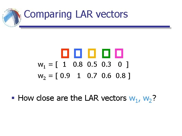
Comparing LAR vectors w 1 = [ 1 0. 8 0. 5 0. 3 0 ] w 2 = [ 0. 9 1 0. 7 0. 6 0. 8 ] § How close are the LAR vectors w 1, w 2?

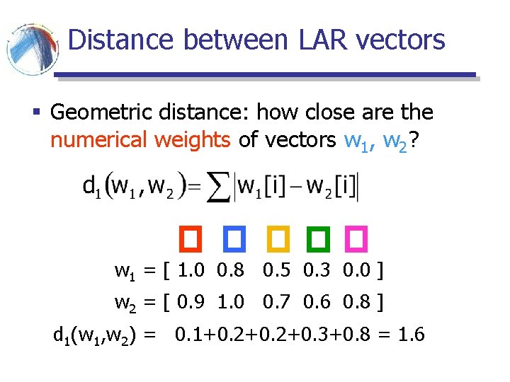
Distance between LAR vectors § Geometric distance: how close are the numerical weights of vectors w 1, w 2? w 1 = [ 1. 0 0. 8 0. 5 0. 3 0. 0 ] w 2 = [ 0. 9 1. 0 0. 7 0. 6 0. 8 ] d 1(w 1, w 2) = 0. 1+0. 2+0. 3+0. 8 = 1. 6

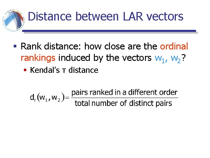
Distance between LAR vectors § Rank distance: how close are the ordinal rankings induced by the vectors w 1, w 2? § Kendal’s τ distance

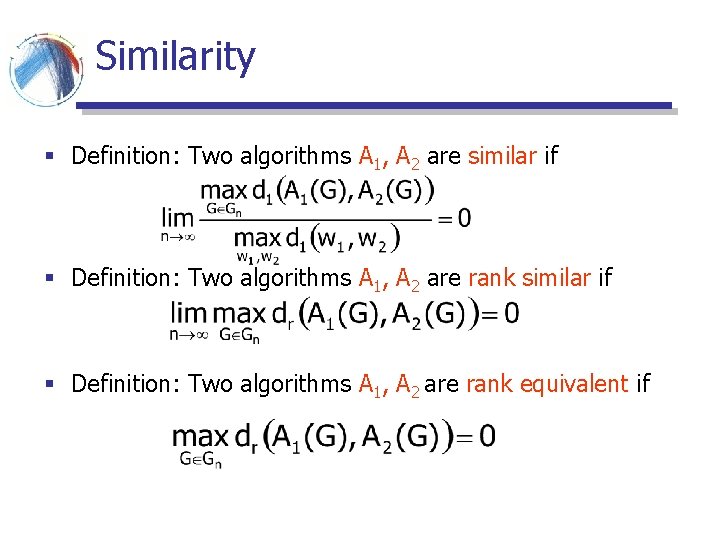
Similarity § Definition: Two algorithms A 1, A 2 are similar if § Definition: Two algorithms A 1, A 2 are rank equivalent if

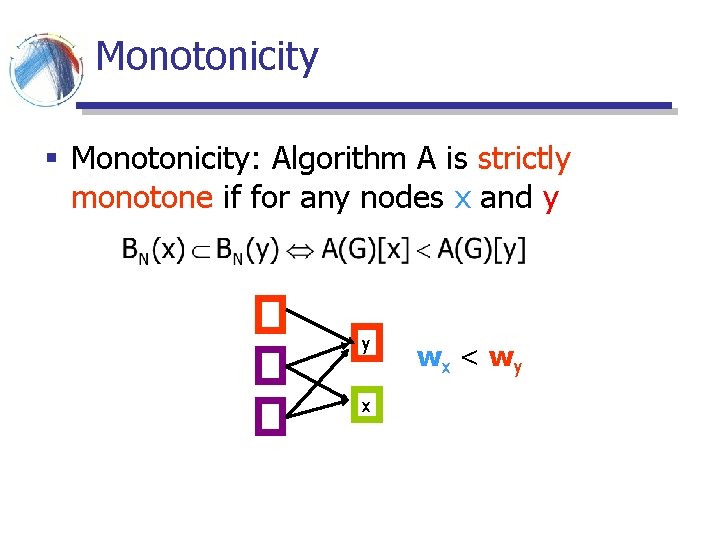
Monotonicity § Monotonicity: Algorithm A is strictly monotone if for any nodes x and y y x wx < wy

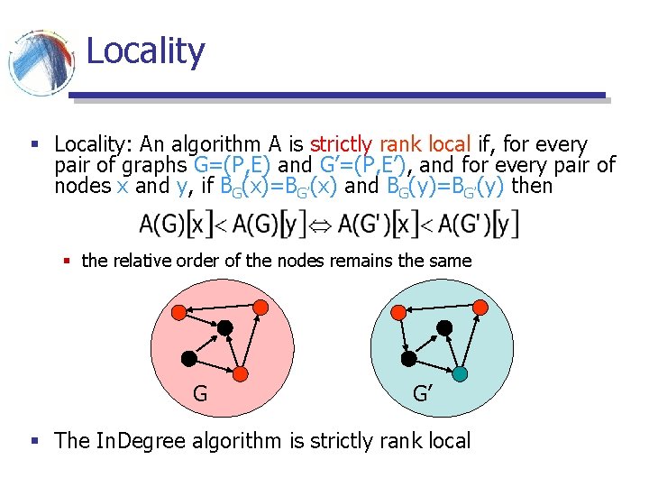
Locality § Locality: An algorithm A is strictly rank local if, for every pair of graphs G=(P, E) and G’=(P, E’), and for every pair of nodes x and y, if BG(x)=BG’(x) and BG(y)=BG’(y) then § the relative order of the nodes remains the same G G’ § The In. Degree algorithm is strictly rank local

Label Independence § Label Independence: An algorithm is label independent if a permutation of the labels of the nodes yields the same permutation of the weights § the weights assigned by the algorithm do not depend on the labels of the nodes

Axiomatic characterization of the In. Degree algorithm [BRRT 05] § Theorem: Any algorithm that is strictly rank local, strictly monotone and label independent is rank equivalent to the In. Degree algorithm

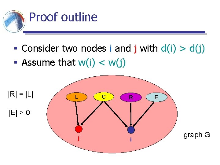
Proof outline § Consider two nodes i and j with d(i) > d(j) § Assume that w(i) < w(j) |R| = |L| L C R E |E| > 0 j i graph G

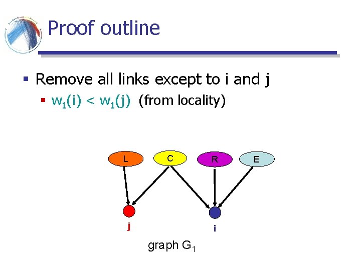
Proof outline § Remove all links except to i and j § w 1(i) < w 1(j) (from locality) L C j R i graph G 1 E

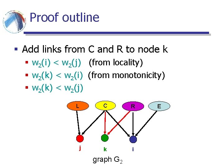
Proof outline § Add links from C and R to node k § w 2(i) < w 2(j) (from locality) § w 2(k) < w 2(i) (from monotonicity) § w 2(k) < w 2(j) L C R j k i graph G 2 E

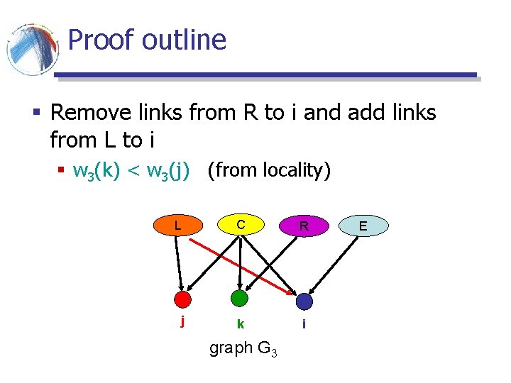
Proof outline § Remove links from R to i and add links from L to i § w 3(k) < w 3(j) (from locality) L C R j k i graph G 3 E

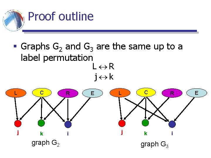
Proof outline § Graphs G 2 and G 3 are the same up to a label permutation L C R j k i graph G 2 E L C R j k i graph G 3 E

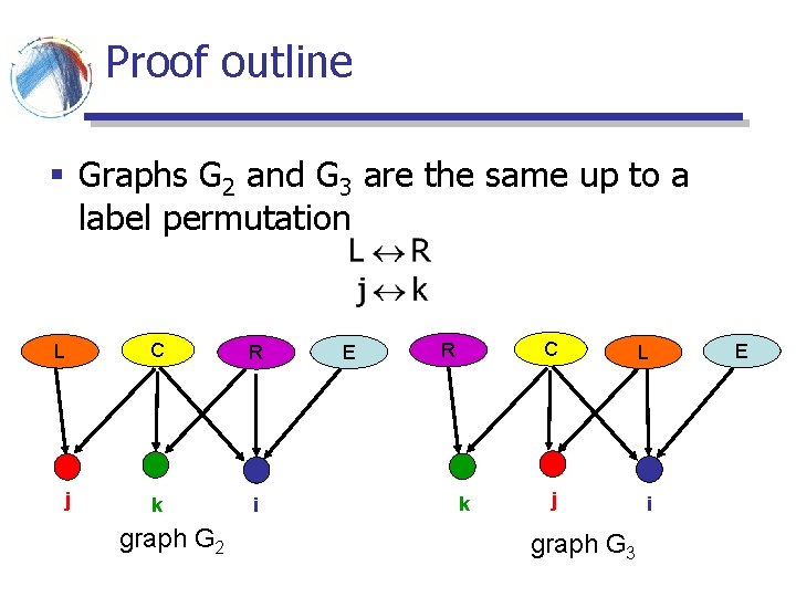
Proof outline § Graphs G 2 and G 3 are the same up to a label permutation L C R j k i graph G 2 E R k C L j i graph G 3 E

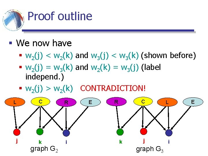
Proof outline § We now have § w 2(j) < w 2(k) and w 3(j) < w 3(k) (shown before) § w 2(j) = w 3(k) and w 2(k) = w 3(j) (label independ. ) § w 2(j) > w 2(k) CONTRADICTION! L C R j k i graph G 2 E R k C L j i graph G 3 E

Axiomatic characterization § All three properties are needed § locality • Page. Rank is also strictly monotone and label independent § monotonicity • consider an algorithm that assigns 1 to nodes with even degree, and 0 to nodes with odd degree § label independence • consider and algorithm that gives the more weight to links that come from some specific page (e. g. the Yahoo page)

Outline § Axiomatic Characterizations of Link Analysis Ranking Algorithms § In. Degree algorithm § Page. Rank algorithm § Rank Aggregation § Computing aggregate scores § Computing aggregate rankings - voting

Self-edge axiom § Algorithm A satisfies the self-edge axiom if the following is true: If page a is ranked at least as high as page b in a graph G(V, E), where a does not have a link to itself, then a should be ranked higher than b in G(V, E U {v, v})

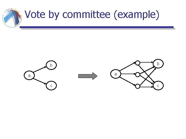
Vote by committee axiom § Algorithm A satisfies the vote by committee axiom if the following is true: If page a links to pages b and c, then the relative ranking of all the pages should be the same as in the case where the direct links from a to b and c are replaced by links from a to a new set of pages which link (only) to b and c

Vote by committee (example) b b a a c c

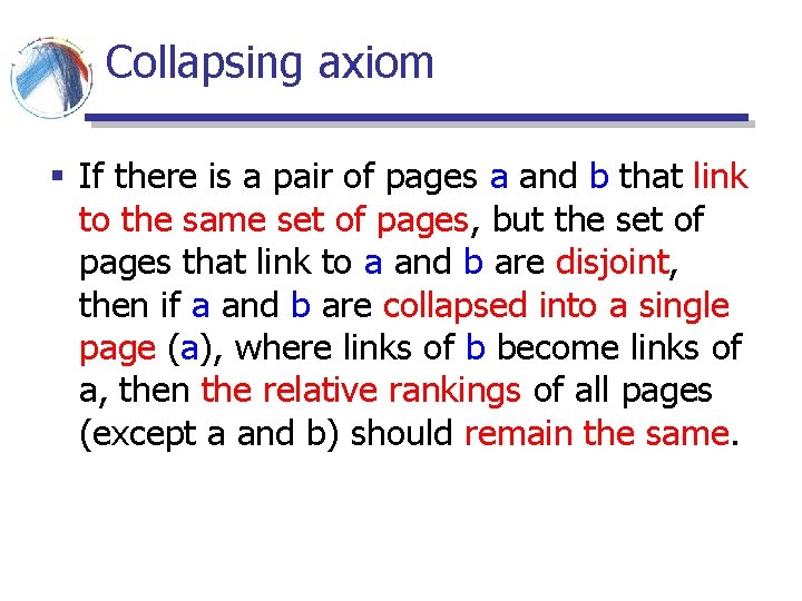
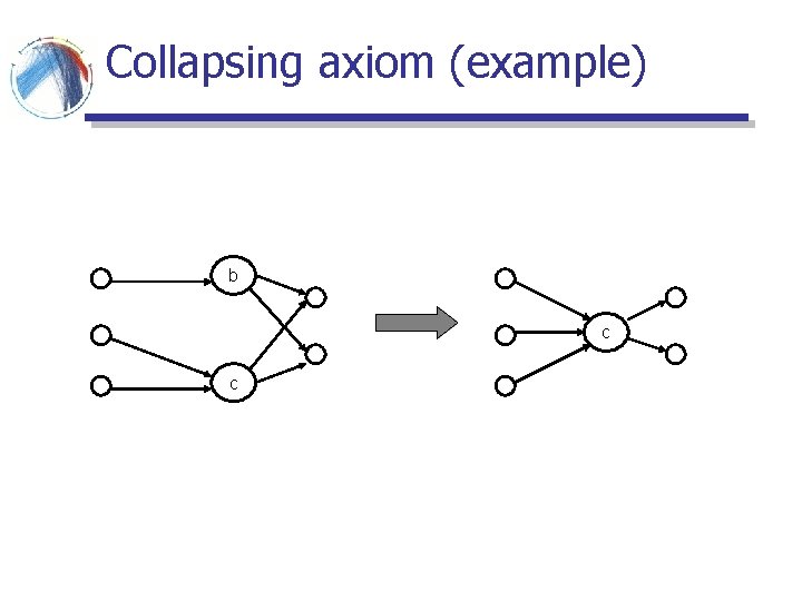
Collapsing axiom § If there is a pair of pages a and b that link to the same set of pages, but the set of pages that link to a and b are disjoint, then if a and b are collapsed into a single page (a), where links of b become links of a, then the relative rankings of all pages (except a and b) should remain the same.

Collapsing axiom (example) b c c

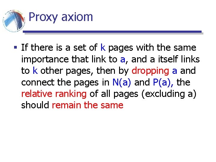
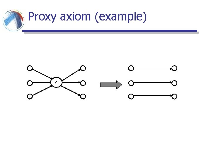
Proxy axiom § If there is a set of k pages with the same importance that link to a, and a itself links to k other pages, then by dropping a and connect the pages in N(a) and P(a), the relative ranking of all pages (excluding a) should remain the same

Proxy axiom (example) c

Axiomatic Characterization of Page. Rank Algorithm [AT 04] § The Page. Rank algorithm satisfies label independence, self-edge, vote by committee, collapsing and proxy axioms.

Outline § Axiomatic Characterizations of Link Analysis Ranking Algorithms § In. Degree algorithm § Page. Rank algorithm § Rank Aggregation § Computing aggregate scores § Computing aggregate rankings - voting

Rank Aggregation § Given a set of rankings R 1, R 2, …, Rm of a set of objects X 1, X 2, …, Xn produce a single ranking R that is in agreement with the existing rankings

Examples § Voting § rankings R 1, R 2, …, Rm are the voters, the objects X 1, X 2, …, Xn are the candidates.

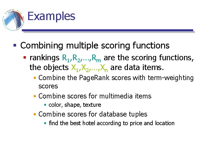
Examples § Combining multiple scoring functions § rankings R 1, R 2, …, Rm are the scoring functions, the objects X 1, X 2, …, Xn are data items. • Combine the Page. Rank scores with term-weighting scores • Combine scores for multimedia items § color, shape, texture • Combine scores for database tuples § find the best hotel according to price and location

Examples § Combining multiple sources § rankings R 1, R 2, …, Rm are the sources, the objects X 1, X 2, …, Xn are data items. • meta-search engines for the Web • distributed databases • P 2 P sources

Variants of the problem § Combining scores § we know the scores assigned to objects by each ranking, and we want to compute a single score § Combining ordinal rankings § the scores are not known, only the ordering is known § the scores are known but we do not know how, or do not want to combine them • e. g. price and star rating

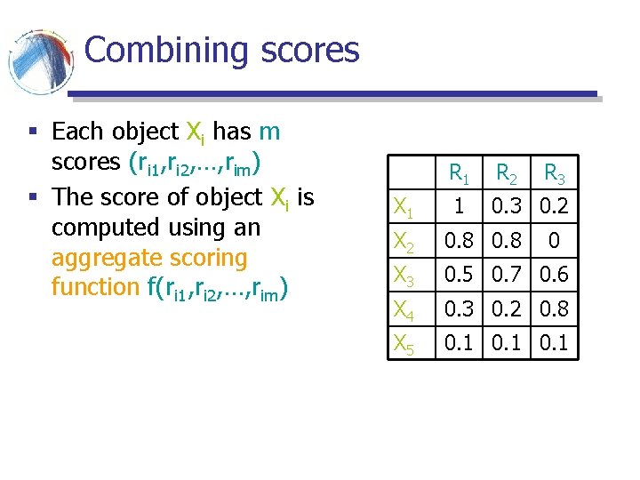
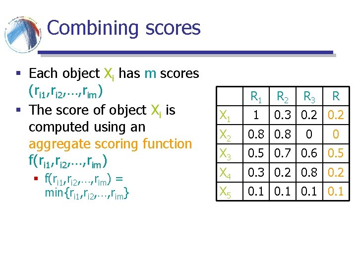
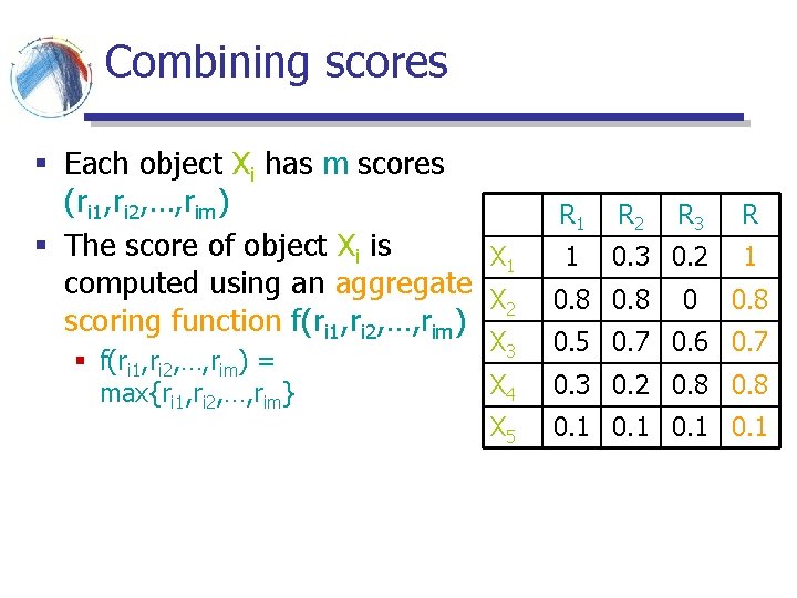
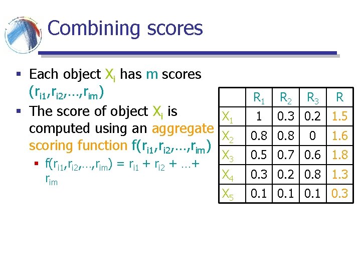
Combining scores § Each object Xi has m scores (ri 1, ri 2, …, rim) § The score of object Xi is computed using an aggregate scoring function f(ri 1, ri 2, …, rim) X 1 R 2 R 3 1 0. 3 0. 2 X 2 0. 8 0 X 3 0. 5 0. 7 0. 6 X 4 0. 3 0. 2 0. 8 X 5 0. 1

Combining scores § Each object Xi has m scores (ri 1, ri 2, …, rim) § The score of object Xi is computed using an aggregate scoring function f(ri 1, ri 2, …, rim) § f(ri 1, ri 2, …, rim) = min{ri 1, ri 2, …, rim} X 1 R 2 R 3 1 0. 3 0. 2 0 R X 2 0. 8 0 X 3 0. 5 0. 7 0. 6 0. 5 X 4 0. 3 0. 2 0. 8 0. 2 X 5 0. 1

Combining scores § Each object Xi has m scores (ri 1, ri 2, …, rim) § The score of object Xi is X 1 computed using an aggregate X scoring function f(ri 1, ri 2, …, rim) 2 § f(ri 1, ri 2, …, rim) = max{ri 1, ri 2, …, rim} R 1 R 2 R 3 R 1 0. 3 0. 2 1 0. 8 0 0. 8 X 3 0. 5 0. 7 0. 6 0. 7 X 4 0. 3 0. 2 0. 8 X 5 0. 1

Combining scores § Each object Xi has m scores (ri 1, ri 2, …, rim) § The score of object Xi is X 1 computed using an aggregate X scoring function f(ri 1, ri 2, …, rim) 2 § f(ri 1, ri 2, …, rim) = ri 1 + ri 2 + …+ rim R 1 R 2 1 0. 3 0. 2 1. 5 0. 8 R 3 0 R 1. 6 X 3 0. 5 0. 7 0. 6 1. 8 X 4 0. 3 0. 2 0. 8 1. 3 X 5 0. 1 0. 3

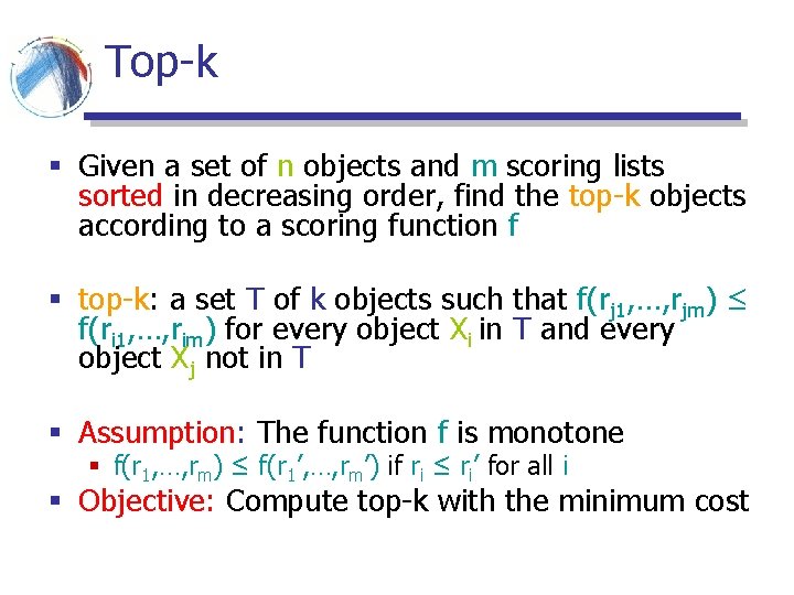
Top-k § Given a set of n objects and m scoring lists sorted in decreasing order, find the top-k objects according to a scoring function f § top-k: a set T of k objects such that f(rj 1, …, rjm) ≤ f(ri 1, …, rim) for every object Xi in T and every object Xj not in T § Assumption: The function f is monotone § f(r 1, …, rm) ≤ f(r 1’, …, rm’) if ri ≤ ri’ for all i § Objective: Compute top-k with the minimum cost

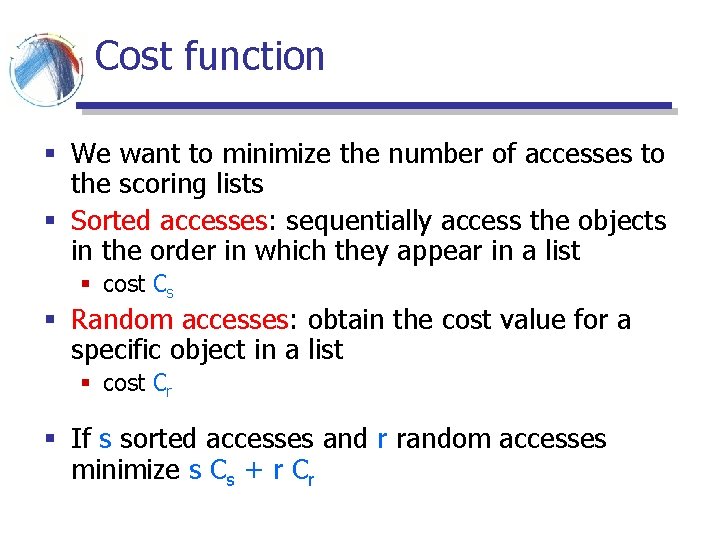
Cost function § We want to minimize the number of accesses to the scoring lists § Sorted accesses: sequentially access the objects in the order in which they appear in a list § cost Cs § Random accesses: obtain the cost value for a specific object in a list § cost Cr § If s sorted accesses and r random accesses minimize s Cs + r Cr

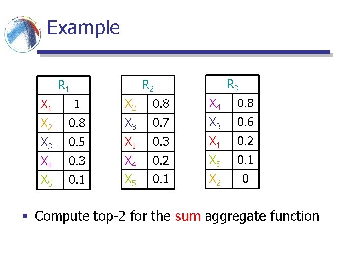
Example R 3 R 2 R 1 X 1 1 X 2 0. 8 X 4 0. 8 X 2 0. 8 X 3 0. 7 X 3 0. 6 X 3 0. 5 X 1 0. 3 X 1 0. 2 X 4 0. 3 X 4 0. 2 X 5 0. 1 X 2 0 § Compute top-2 for the sum aggregate function

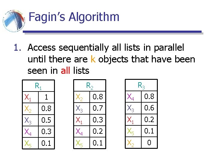
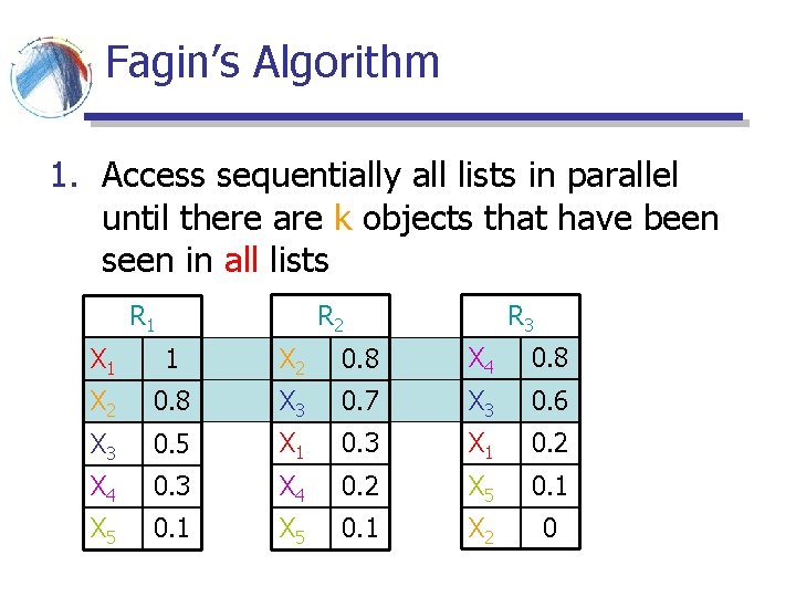
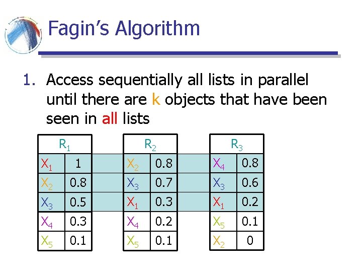
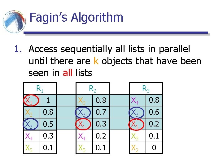
Fagin’s Algorithm 1. Access sequentially all lists in parallel until there are k objects that have been seen in all lists R 3 R 2 R 1 X 1 1 X 2 0. 8 X 4 0. 8 X 2 0. 8 X 3 0. 7 X 3 0. 6 X 3 0. 5 X 1 0. 3 X 1 0. 2 X 4 0. 3 X 4 0. 2 X 5 0. 1 X 2 0

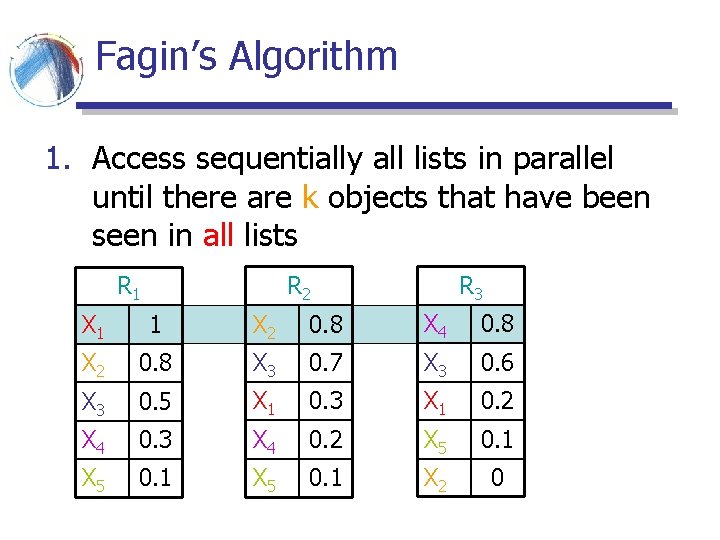
Fagin’s Algorithm 1. Access sequentially all lists in parallel until there are k objects that have been seen in all lists R 3 R 2 R 1 X 1 1 X 2 0. 8 X 4 0. 8 X 2 0. 8 X 3 0. 7 X 3 0. 6 X 3 0. 5 X 1 0. 3 X 1 0. 2 X 4 0. 3 X 4 0. 2 X 5 0. 1 X 2 0

Fagin’s Algorithm 1. Access sequentially all lists in parallel until there are k objects that have been seen in all lists R 3 R 2 R 1 X 1 1 X 2 0. 8 X 4 0. 8 X 2 0. 8 X 3 0. 7 X 3 0. 6 X 3 0. 5 X 1 0. 3 X 1 0. 2 X 4 0. 3 X 4 0. 2 X 5 0. 1 X 2 0

Fagin’s Algorithm 1. Access sequentially all lists in parallel until there are k objects that have been seen in all lists R 3 R 2 R 1 X 1 1 X 2 0. 8 X 4 0. 8 X 2 0. 8 X 3 0. 7 X 3 0. 6 X 3 0. 5 X 1 0. 3 X 1 0. 2 X 4 0. 3 X 4 0. 2 X 5 0. 1 X 2 0

Fagin’s Algorithm 1. Access sequentially all lists in parallel until there are k objects that have been seen in all lists R 3 R 2 R 1 X 1 1 X 2 0. 8 X 4 0. 8 X 2 0. 8 X 3 0. 7 X 3 0. 6 X 3 0. 5 X 1 0. 3 X 1 0. 2 X 4 0. 3 X 4 0. 2 X 5 0. 1 X 2 0

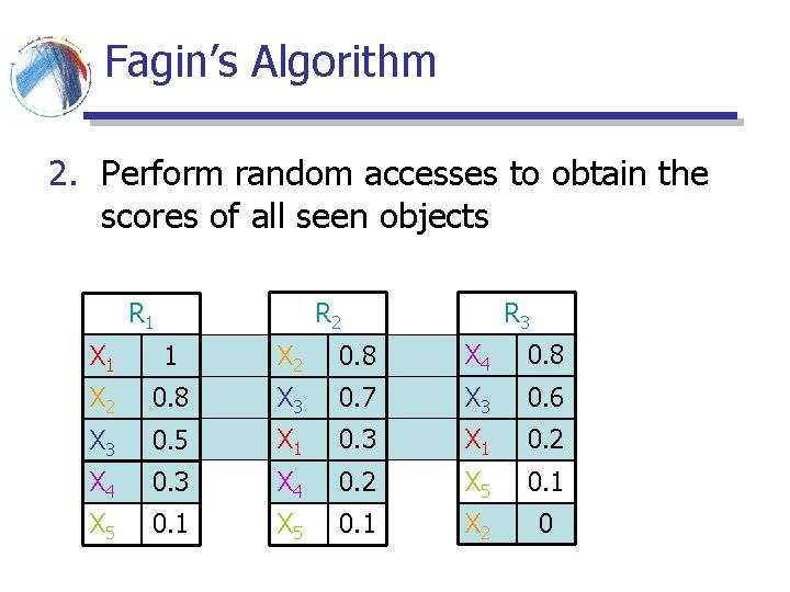
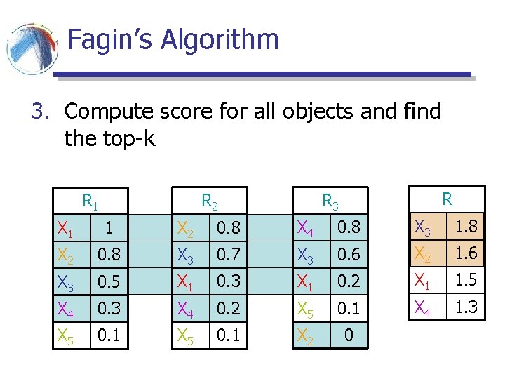
Fagin’s Algorithm 2. Perform random accesses to obtain the scores of all seen objects R 3 R 2 R 1 X 1 1 X 2 0. 8 X 4 0. 8 X 2 0. 8 X 3 0. 7 X 3 0. 6 X 3 0. 5 X 1 0. 3 X 1 0. 2 X 4 0. 3 X 4 0. 2 X 5 0. 1 X 2 0

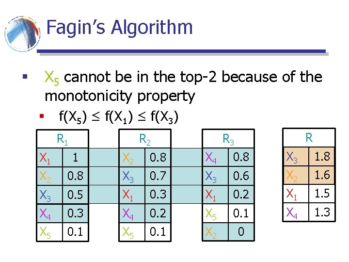
Fagin’s Algorithm 3. Compute score for all objects and find the top-k R R 3 R 2 R 1 X 1 1 X 2 0. 8 X 4 0. 8 X 3 1. 8 X 2 0. 8 X 3 0. 7 X 3 0. 6 X 2 1. 6 X 3 0. 5 X 1 0. 3 X 1 0. 2 X 1 1. 5 X 4 0. 3 X 4 0. 2 X 5 0. 1 X 4 1. 3 X 5 0. 1 X 2 0

Fagin’s Algorithm § X 5 cannot be in the top-2 because of the monotonicity property § f(X 5) ≤ f(X 1) ≤ f(X 3) R R 3 R 2 R 1 X 1 1 X 2 0. 8 X 4 0. 8 X 3 1. 8 X 2 0. 8 X 3 0. 7 X 3 0. 6 X 2 1. 6 X 3 0. 5 X 1 0. 3 X 1 0. 2 X 1 1. 5 X 4 0. 3 X 4 0. 2 X 5 0. 1 X 4 1. 3 X 5 0. 1 X 2 0

Fagin’s Algorithm § The algorithm is cost optimal under some probabilistic assumptions for a restricted class of aggregate functions

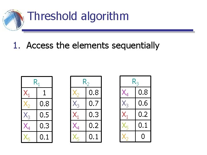
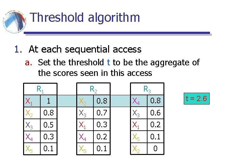
Threshold algorithm 1. Access the elements sequentially R 3 R 2 R 1 X 1 1 X 2 0. 8 X 4 0. 8 X 2 0. 8 X 3 0. 7 X 3 0. 6 X 3 0. 5 X 1 0. 3 X 1 0. 2 X 4 0. 3 X 4 0. 2 X 5 0. 1 X 2 0

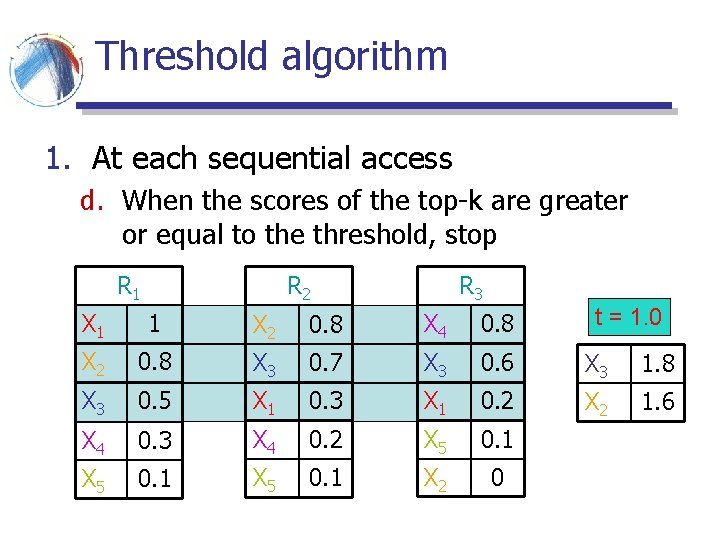
Threshold algorithm 1. At each sequential access a. Set the threshold t to be the aggregate of the scores seen in this access R 3 R 2 R 1 X 1 1 X 2 0. 8 X 4 0. 8 X 2 0. 8 X 3 0. 7 X 3 0. 6 X 3 0. 5 X 1 0. 3 X 1 0. 2 X 4 0. 3 X 4 0. 2 X 5 0. 1 X 2 0 t = 2. 6

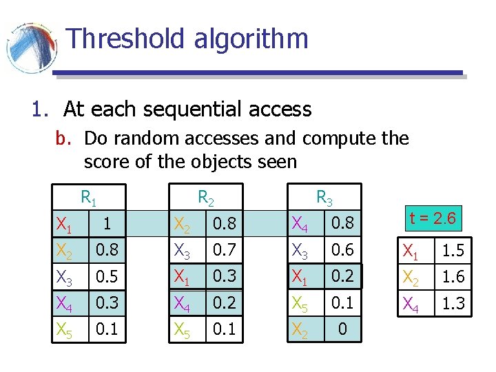
Threshold algorithm 1. At each sequential access b. Do random accesses and compute the score of the objects seen R 3 R 2 R 1 t = 2. 6 X 1 1 X 2 0. 8 X 4 0. 8 X 2 0. 8 X 3 0. 7 X 3 0. 6 X 1 1. 5 X 3 0. 5 X 1 0. 3 X 1 0. 2 X 2 1. 6 X 4 0. 3 X 4 0. 2 X 5 0. 1 X 4 1. 3 X 5 0. 1 X 2 0

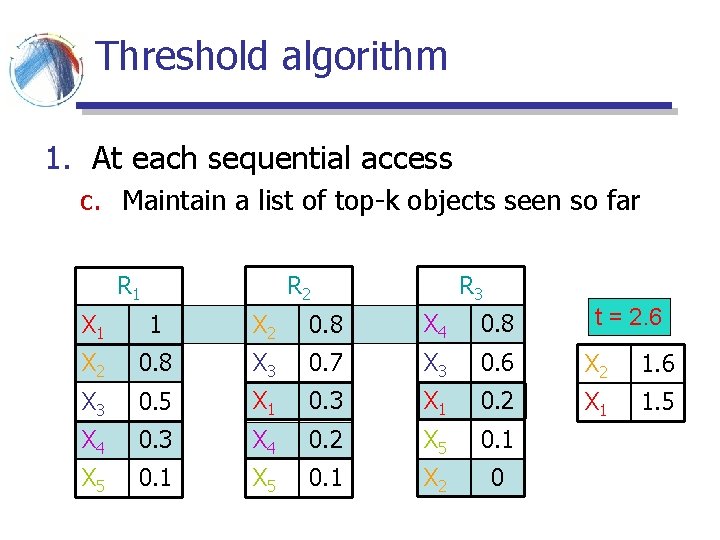
Threshold algorithm 1. At each sequential access c. Maintain a list of top-k objects seen so far R 3 R 2 R 1 t = 2. 6 X 1 1 X 2 0. 8 X 4 0. 8 X 2 0. 8 X 3 0. 7 X 3 0. 6 X 2 1. 6 X 3 0. 5 X 1 0. 3 X 1 0. 2 X 1 1. 5 X 4 0. 3 X 4 0. 2 X 5 0. 1 X 2 0

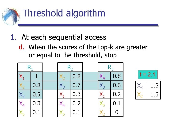
Threshold algorithm 1. At each sequential access d. When the scores of the top-k are greater or equal to the threshold, stop R 3 R 2 R 1 t = 2. 1 X 1 1 X 2 0. 8 X 4 0. 8 X 2 0. 8 X 3 0. 7 X 3 0. 6 X 3 1. 8 X 3 0. 5 X 1 0. 3 X 1 0. 2 X 2 1. 6 X 4 0. 3 X 4 0. 2 X 5 0. 1 X 2 0

Threshold algorithm 1. At each sequential access d. When the scores of the top-k are greater or equal to the threshold, stop R 1 R 3 R 2 t = 1. 0 X 1 1 X 2 0. 8 X 4 0. 8 X 2 0. 8 X 3 0. 7 X 3 0. 6 X 3 1. 8 X 3 0. 5 X 1 0. 3 X 1 0. 2 X 2 1. 6 X 4 0. 3 X 4 0. 2 X 5 0. 1 X 2 0

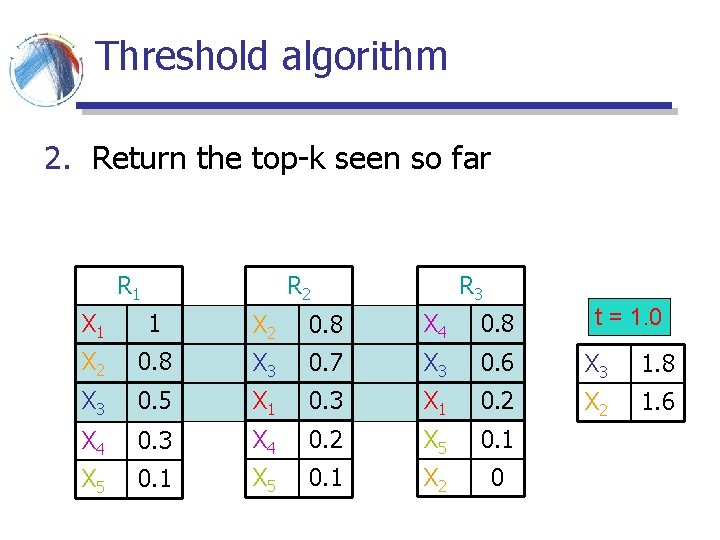
Threshold algorithm 2. Return the top-k seen so far R 1 R 3 R 2 t = 1. 0 X 1 1 X 2 0. 8 X 4 0. 8 X 2 0. 8 X 3 0. 7 X 3 0. 6 X 3 1. 8 X 3 0. 5 X 1 0. 3 X 1 0. 2 X 2 1. 6 X 4 0. 3 X 4 0. 2 X 5 0. 1 X 2 0

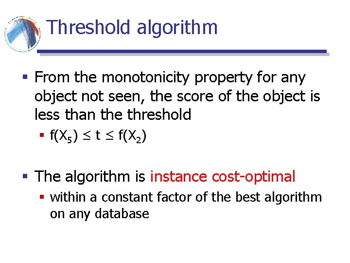
Threshold algorithm § From the monotonicity property for any object not seen, the score of the object is less than the threshold § f(X 5) ≤ t ≤ f(X 2) § The algorithm is instance cost-optimal § within a constant factor of the best algorithm on any database

Combining rankings § In many cases the scores are not known § e. g. meta-search engines – scores are proprietary information § … or we do not know how they were obtained § one search engine returns score 10, the other 100. What does this mean? § … or the scores are incompatible § apples and oranges: does it make sense to combine price with distance? § In this cases we can only work with the rankings

The problem § Input: a set of rankings R 1, R 2, …, Rm of the objects X 1, X 2, …, Xn. Each ranking Ri is a total ordering of the objects § for every pair Xi, Xj either Xi is ranked above Xj or Xj is ranked above Xi § Output: A total ordering R that aggregates rankings R 1, R 2, …, Rm

Voting theory § A voting system is a rank aggregation mechanism § Long history and literature § criteria and axioms for good voting systems

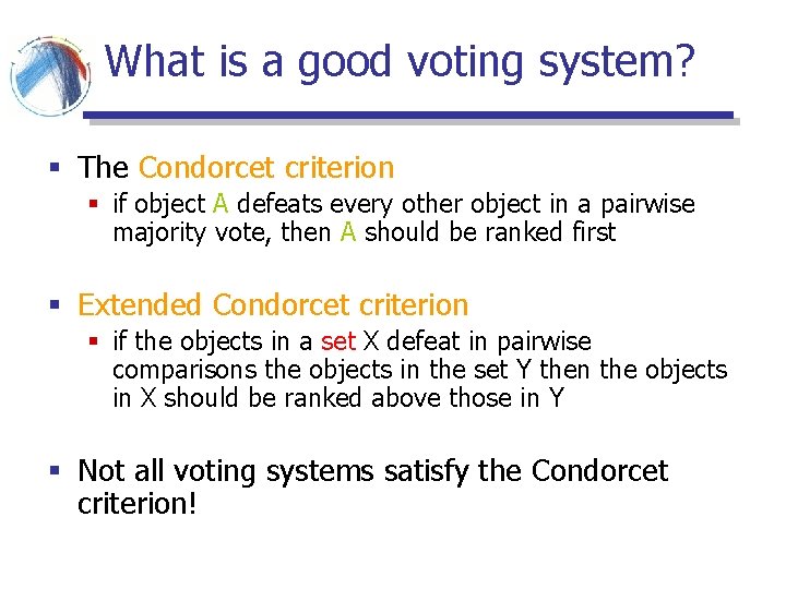
What is a good voting system? § The Condorcet criterion § if object A defeats every other object in a pairwise majority vote, then A should be ranked first § Extended Condorcet criterion § if the objects in a set X defeat in pairwise comparisons the objects in the set Y then the objects in X should be ranked above those in Y § Not all voting systems satisfy the Condorcet criterion!

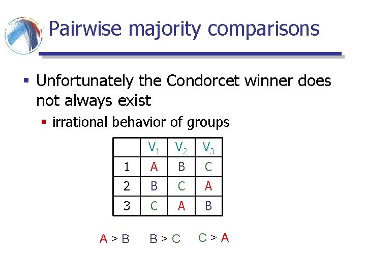
Pairwise majority comparisons § Unfortunately the Condorcet winner does not always exist § irrational behavior of groups V 1 V 2 V 3 1 A B C 2 B C A 3 C A B A>B B>C C>A

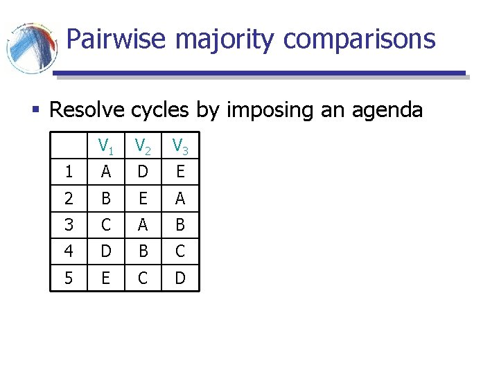
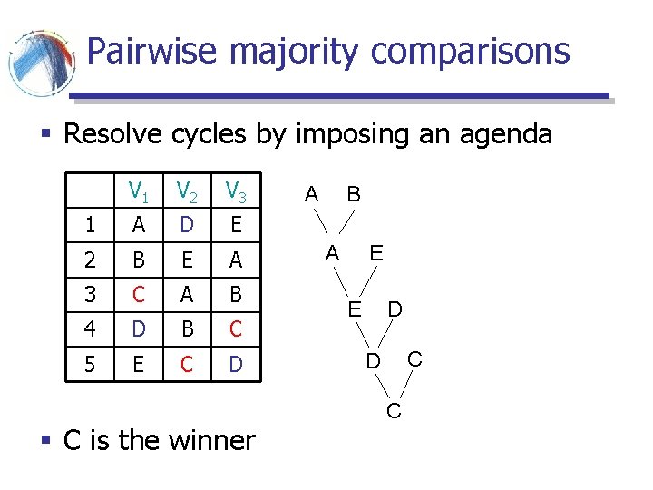
Pairwise majority comparisons § Resolve cycles by imposing an agenda V 1 V 2 V 3 1 A D E 2 B E A 3 C A B 4 D B C 5 E C D

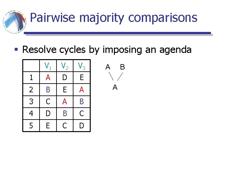
Pairwise majority comparisons § Resolve cycles by imposing an agenda V 1 V 2 V 3 1 A D E 2 B E A 3 C A B 4 D B C 5 E C D B A A

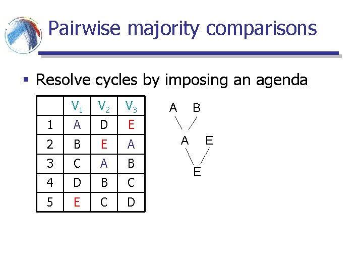
Pairwise majority comparisons § Resolve cycles by imposing an agenda V 1 V 2 V 3 1 A D E 2 B E A 3 C A B 4 D B C 5 E C D B A E

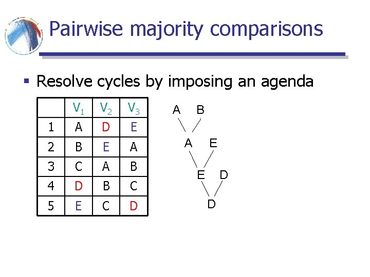
Pairwise majority comparisons § Resolve cycles by imposing an agenda V 1 V 2 V 3 1 A D E 2 B E A 3 C A B 4 D B C 5 E C D B A E A D E D

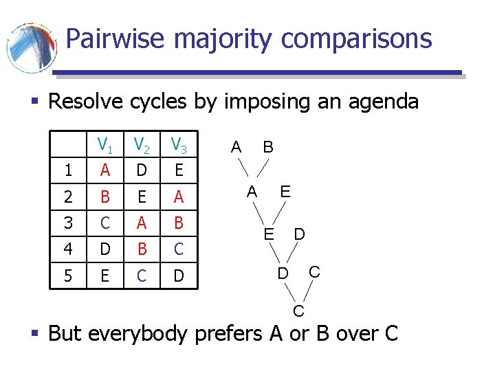
Pairwise majority comparisons § Resolve cycles by imposing an agenda V 1 V 2 V 3 1 A D E 2 B E A 3 C A B 4 D B C 5 E C D § C is the winner B A E A D E C D C

Pairwise majority comparisons § Resolve cycles by imposing an agenda V 1 V 2 V 3 1 A D E 2 B E A 3 C A B 4 D B C 5 E C D B A E A D E C D C § But everybody prefers A or B over C

Pairwise majority comparisons § The voting system is not Pareto optimal § there exists another ordering that everybody prefers § Also, it is sensitive to the order of voting

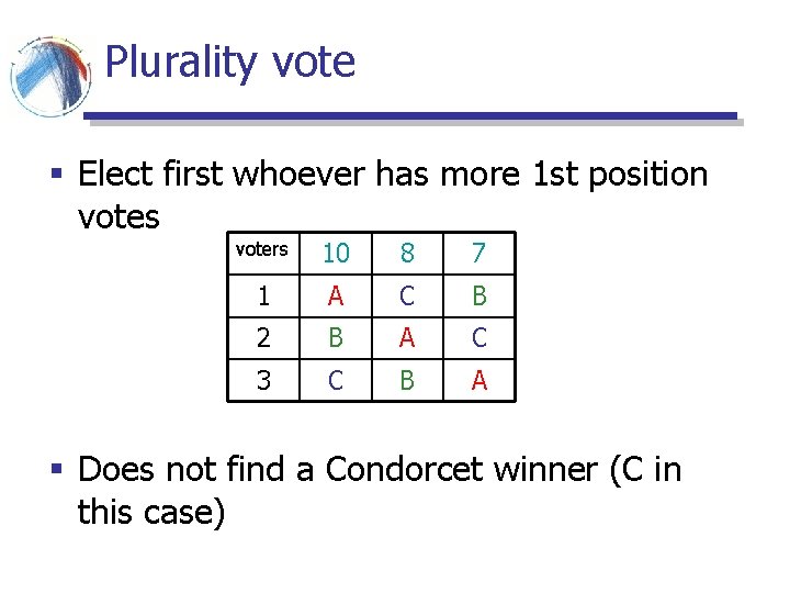
Plurality vote § Elect first whoever has more 1 st position votes voters 10 8 7 1 A C B 2 B A C 3 C B A § Does not find a Condorcet winner (C in this case)

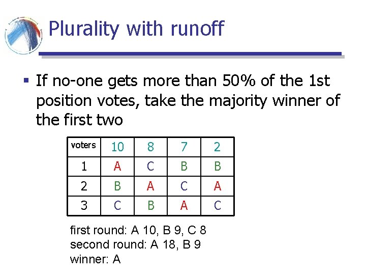
Plurality with runoff § If no-one gets more than 50% of the 1 st position votes, take the majority winner of the first two voters 10 8 7 2 1 A C B B 2 B A C A 3 C B A C first round: A 10, B 9, C 8 second round: A 18, B 9 winner: A

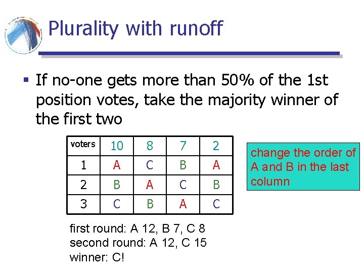
Plurality with runoff § If no-one gets more than 50% of the 1 st position votes, take the majority winner of the first two voters 10 8 7 2 1 A C B A 2 B A C B 3 C B A C first round: A 12, B 7, C 8 second round: A 12, C 15 winner: C! change the order of A and B in the last column

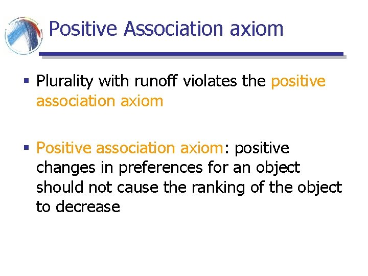
Positive Association axiom § Plurality with runoff violates the positive association axiom § Positive association axiom: positive changes in preferences for an object should not cause the ranking of the object to decrease

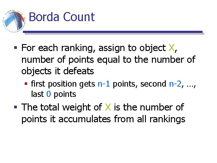
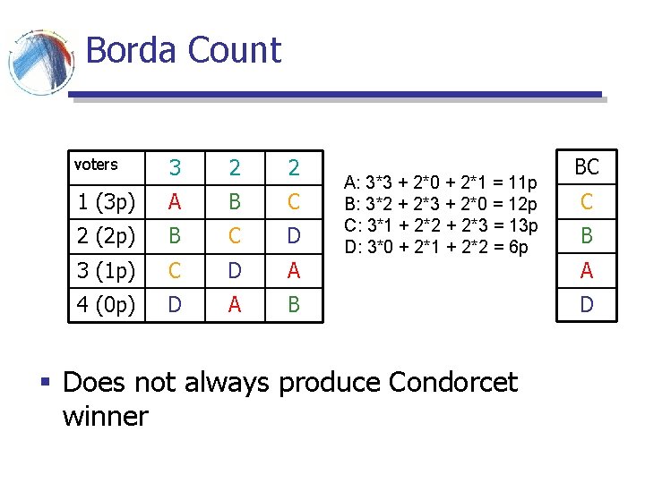
Borda Count § For each ranking, assign to object X, number of points equal to the number of objects it defeats § first position gets n-1 points, second n-2, …, last 0 points § The total weight of X is the number of points it accumulates from all rankings

Borda Count voters 3 2 2 1 (3 p) A B C 2 (2 p) B C D 3 (1 p) C D A 4 (0 p) D A B A: 3*3 + 2*0 + 2*1 = 11 p B: 3*2 + 2*3 + 2*0 = 12 p C: 3*1 + 2*2 + 2*3 = 13 p D: 3*0 + 2*1 + 2*2 = 6 p § Does not always produce Condorcet winner BC C B A D

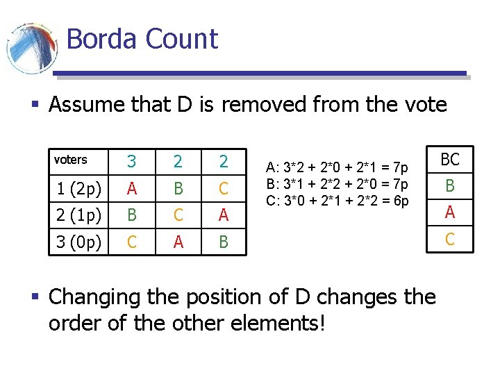
Borda Count § Assume that D is removed from the voters 3 2 2 1 (2 p) A B C 2 (1 p) B C A 3 (0 p) C A B A: 3*2 + 2*0 + 2*1 = 7 p B: 3*1 + 2*2 + 2*0 = 7 p C: 3*0 + 2*1 + 2*2 = 6 p § Changing the position of D changes the order of the other elements! BC B A C

Independence of Irrelevant Alternatives § The relative ranking of X and Y should not depend on a third object Z § heavily debated axiom

Borda Count § The Borda Count of an an object X is the aggregate number of pairwise comparisons that the object X wins § follows from the fact that in one ranking X wins all the pairwise comparisons with objects that are under X in the ranking

Voting Theory § Is there a voting system that does not suffer from the previous shortcomings?

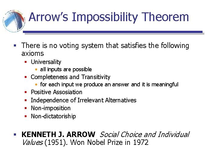
Arrow’s Impossibility Theorem § There is no voting system that satisfies the following axioms § Universality • all inputs are possible § Completeness and Transitivity • for each input we produce an answer and it is meaningful § § Positive Assosiation Independence of Irrelevant Alternatives Non-imposition Non-dictatoriship § KENNETH J. ARROW Social Choice and Individual Values (1951). Won Nobel Prize in 1972

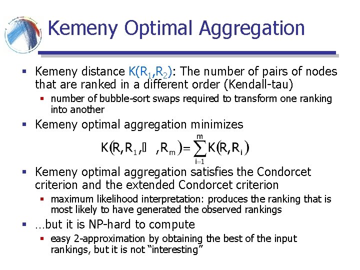
Kemeny Optimal Aggregation § Kemeny distance K(R 1, R 2): The number of pairs of nodes that are ranked in a different order (Kendall-tau) § number of bubble-sort swaps required to transform one ranking into another § Kemeny optimal aggregation minimizes § Kemeny optimal aggregation satisfies the Condorcet criterion and the extended Condorcet criterion § maximum likelihood interpretation: produces the ranking that is most likely to have generated the observed rankings § …but it is NP-hard to compute § easy 2 -approximation by obtaining the best of the input rankings, but it is not “interesting”

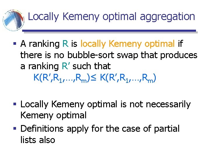
Locally Kemeny optimal aggregation § A ranking R is locally Kemeny optimal if there is no bubble-sort swap that produces a ranking R’ such that K(R’, R 1, …, Rm)≤ K(R’, R 1, …, Rm) § Locally Kemeny optimal is not necessarily Kemeny optimal § Definitions apply for the case of partial lists also

Locally Kemeny optimal aggregation § Locally Kemeny optimal aggregation can be computed in polynomial time § At the i-th iteration insert the i-th element x in the bottom of the list, and bubble it up until there is an element y such that the majority places y over x § Locally Kemeny optimal aggregation satisfies the Condorcet and extended Condorcet criterion

Rank Aggregation algorithm [DKNS 01] § Start with an aggregated ranking and make it into a locally Kemeny optimal aggregation § How do we select the initial aggregation? § Use another aggregation method § Create a Markov Chain where you move from an object X, to another object Y that is ranked higher by the majority

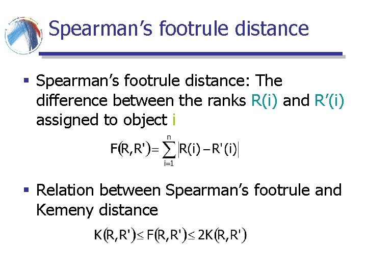
Spearman’s footrule distance § Spearman’s footrule distance: The difference between the ranks R(i) and R’(i) assigned to object i § Relation between Spearman’s footrule and Kemeny distance

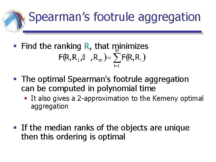
Spearman’s footrule aggregation § Find the ranking R, that minimizes § The optimal Spearman’s footrule aggregation can be computed in polynomial time § It also gives a 2 -approximation to the Kemeny optimal aggregation § If the median ranks of the objects are unique then this ordering is optimal

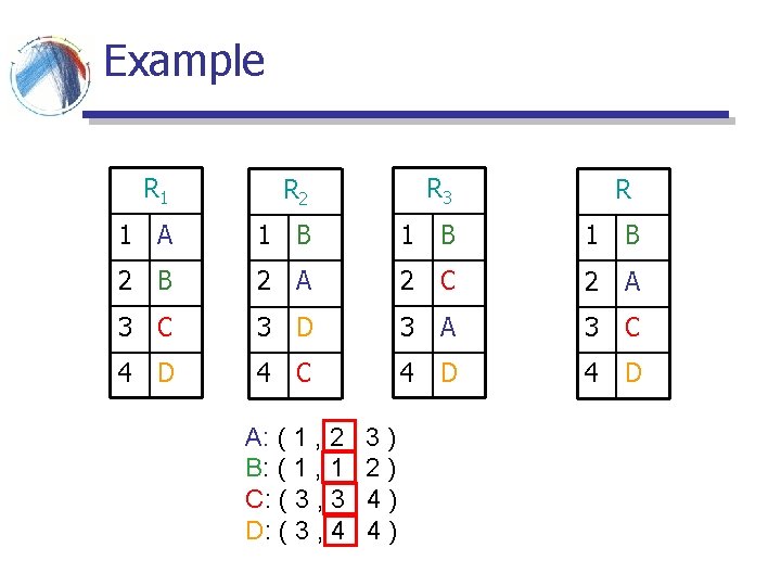
Example R 1 R 2 R 3 1 A 1 B 1 B 2 A 2 C 2 A 3 C 3 D 3 A 3 C 4 D 4 D A: ( 1 , 2 , 3 ) B: ( 1 , 2 ) C: ( 3 , 4 ) D: ( 3 , 4 ) R

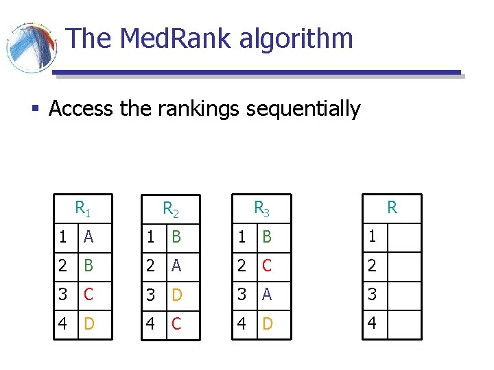
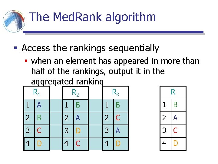
The Med. Rank algorithm § Access the rankings sequentially R R 1 R 2 R 3 1 A 1 B 1 2 B 2 A 2 C 2 3 C 3 D 3 A 3 4 D 4 C 4 D 4

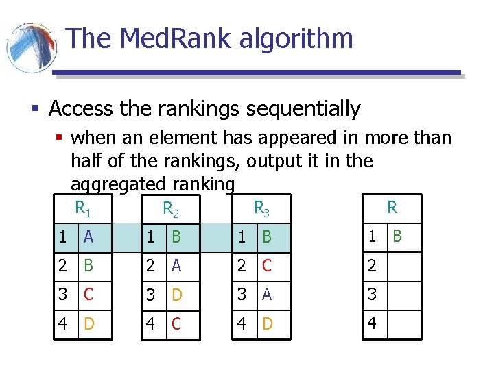
The Med. Rank algorithm § Access the rankings sequentially § when an element has appeared in more than half of the rankings, output it in the aggregated ranking R R 1 R 2 R 3 1 A 1 B 1 B 2 A 2 C 2 3 C 3 D 3 A 3 4 D 4 C 4 D 4

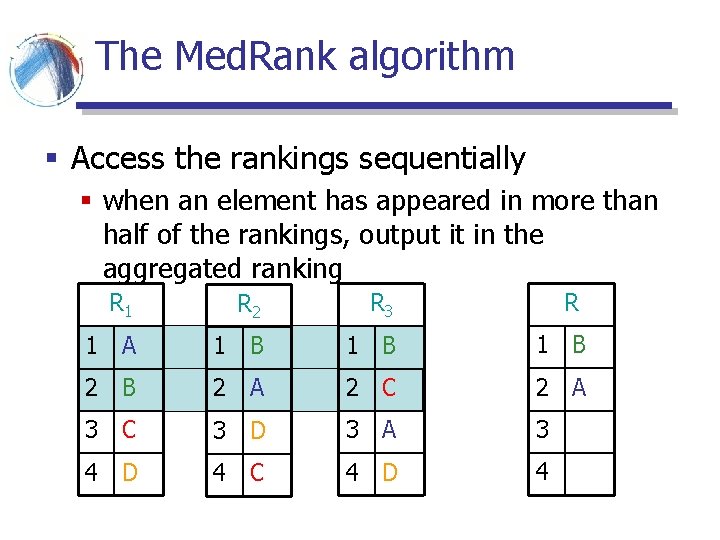
The Med. Rank algorithm § Access the rankings sequentially § when an element has appeared in more than half of the rankings, output it in the aggregated ranking R R 1 R 2 R 3 1 A 1 B 1 B 2 A 2 C 2 A 3 C 3 D 3 A 3 4 D 4 C 4 D 4

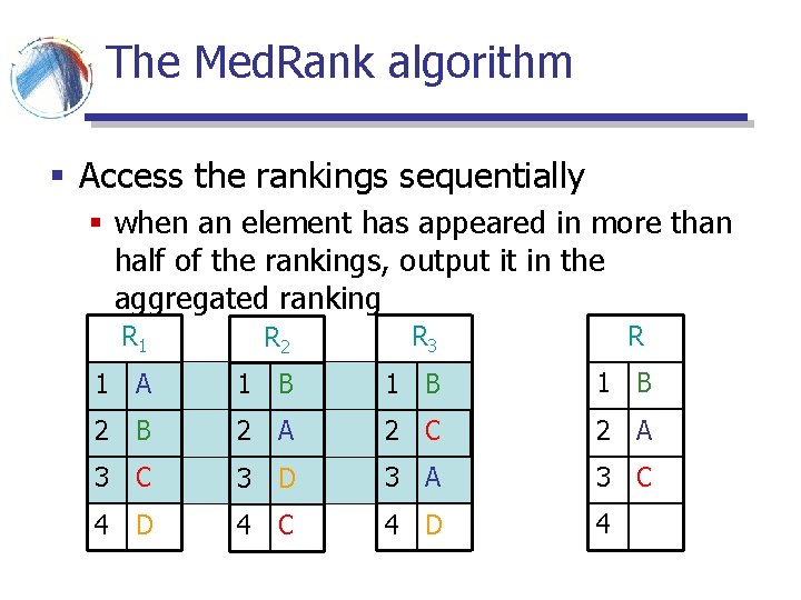
The Med. Rank algorithm § Access the rankings sequentially § when an element has appeared in more than half of the rankings, output it in the aggregated ranking R R 1 R 2 R 3 1 A 1 B 1 B 2 A 2 C 2 A 3 C 3 D 3 A 3 C 4 D 4

The Med. Rank algorithm § Access the rankings sequentially § when an element has appeared in more than half of the rankings, output it in the aggregated ranking R R 1 R 2 R 3 1 A 1 B 1 B 2 A 2 C 2 A 3 C 3 D 3 A 3 C 4 D 4 D

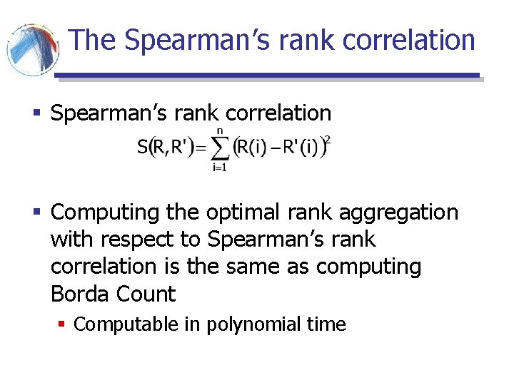
The Spearman’s rank correlation § Computing the optimal rank aggregation with respect to Spearman’s rank correlation is the same as computing Borda Count § Computable in polynomial time

Extensions and Applications § Rank distance measures between partial orderings and top-k lists § Similarity search § Ranked Join Indices § Analysis of Link Analysis Ranking algorithms § Connections with machine learning

References § § § § A. Borodin, G. Roberts, J. Rosenthal, P. Tsaparas, Link Analysis Ranking: Algorithms, Theory and Experiments, ACM Transactions on Internet Technologies (TOIT), 5(1), 2005 Ron Fagin, Ravi Kumar, Mohammad Mahdian, D. Sivakumar, Erik Vee, Comparing and aggregating rankings with ties , PODS 2004 M. Tennenholtz, and Alon Altman, "On the Axiomatic Foundations of Ranking Systems", Proceedings of IJCAI, 2005 Ron Fagin, Amnon Lotem, Moni Naor. Optimal aggregation algorithms for middleware, J. Computer and System Sciences 66 (2003), pp. 614 -656. Extended abstract appeared in Proc. 2001 ACM Symposium on Principles of Database Systems (PODS '01), pp. 102 -113. Alex Tabbarok Lecture Notes Ron Fagin, Ravi Kumar, D. Sivakumar Efficient similarity search and classification via rank aggregation, Proc. 2003 ACM SIGMOD Conference (SIGMOD '03), pp. 301 -312. Cynthia Dwork, Ravi Kumar, Moni Naor, D. Sivakumar. Rank Aggregation Methods for the Web. 10 th International World Wide Web Conference, May 2001. C. Dwork, R. Kumar, M. Naor, D. Sivakumar, "Rank Aggregation Revisited, " WWW 10; selected as Web Search Area highlight, 2001.