Models and Algorithms for Complex Networks Network models

Models and Algorithms for Complex Networks Network models

What is a network model? § Informally, a network model is a process (radomized or deterministic) for generating a graph § Models of static graphs § input: a set of parameters Π, and the size of the graph n § output: a graph G(Π, n) § Models of evolving graphs § input: a set of parameters Π, and an initial graph G 0 § output: a graph Gt for each time t

Families of random graphs § A deterministic model D defines a single graph for each value of n (or t) § A randomized model R defines a probability space ‹Gn, P› where Gn is the set of all graphs of size n, and P a probability distribution over the set Gn (similarly for t) § we call this a family of random graphs R, or a random graph R

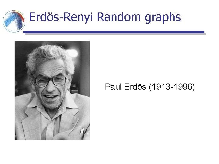
Erdös-Renyi Random graphs Paul Erdös (1913 -1996)

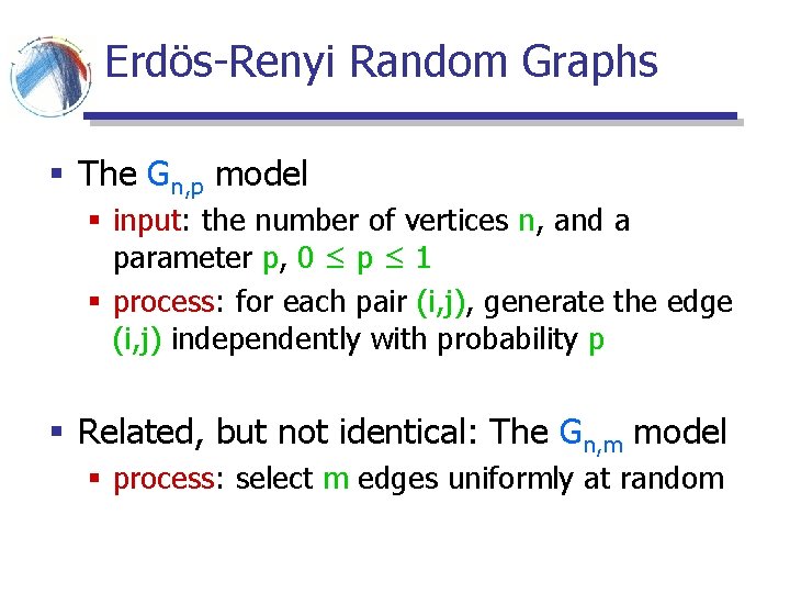
Erdös-Renyi Random Graphs § The Gn, p model § input: the number of vertices n, and a parameter p, 0 ≤ p ≤ 1 § process: for each pair (i, j), generate the edge (i, j) independently with probability p § Related, but not identical: The Gn, m model § process: select m edges uniformly at random

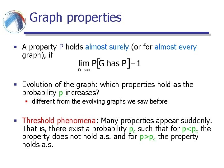
Graph properties § A property P holds almost surely (or for almost every graph), if § Evolution of the graph: which properties hold as the probability p increases? § different from the evolving graphs we saw before § Threshold phenomena: Many properties appear suddenly. That is, there exist a probability pc such that for p<pc the property does not hold a. s. and for p>pc the property holds a. s.

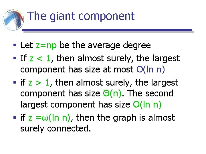
The giant component § Let z=np be the average degree § If z < 1, then almost surely, the largest component has size at most O(ln n) § if z > 1, then almost surely, the largest component has size Θ(n). The second largest component has size O(ln n) § if z =ω(ln n), then the graph is almost surely connected.

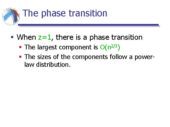
The phase transition § When z=1, there is a phase transition § The largest component is O(n 2/3) § The sizes of the components follow a powerlaw distribution.

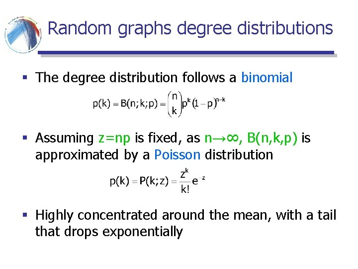
Random graphs degree distributions § The degree distribution follows a binomial § Assuming z=np is fixed, as n→∞, B(n, k, p) is approximated by a Poisson distribution § Highly concentrated around the mean, with a tail that drops exponentially

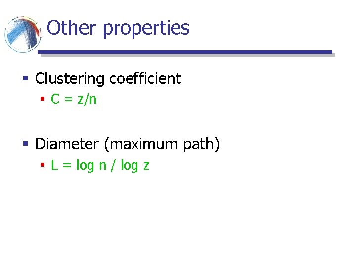
Other properties § Clustering coefficient § C = z/n § Diameter (maximum path) § L = log n / log z

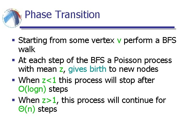
Phase Transition § Starting from some vertex v perform a BFS walk § At each step of the BFS a Poisson process with mean z, gives birth to new nodes § When z<1 this process will stop after O(logn) steps § When z>1, this process will continue for Θ(n) steps

Random graphs and real life § A beautiful and elegant theory studied exhaustively § Random graphs had been used as idealized network models § Unfortunately, they don’t capture reality…

Departing from the ER model § We need models that better capture the characteristics of real graphs § degree sequences § clustering coefficient § short paths

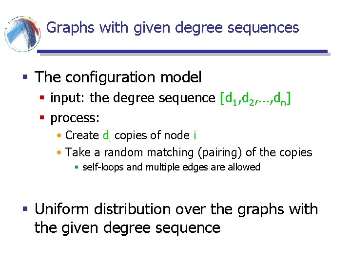
Graphs with given degree sequences § The configuration model § input: the degree sequence [d 1, d 2, …, dn] § process: • Create di copies of node i • Take a random matching (pairing) of the copies § self-loops and multiple edges are allowed § Uniform distribution over the graphs with the given degree sequence

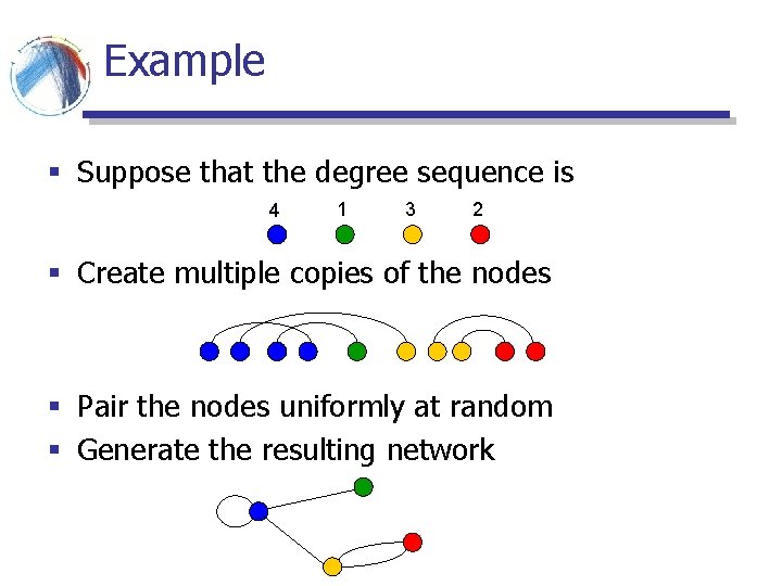
Example § Suppose that the degree sequence is 4 1 3 2 § Create multiple copies of the nodes § Pair the nodes uniformly at random § Generate the resulting network

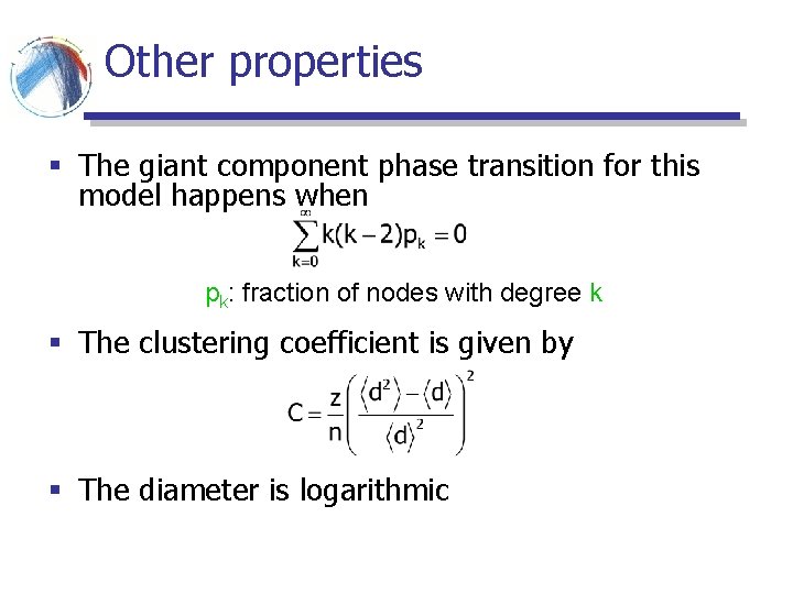
Other properties § The giant component phase transition for this model happens when pk: fraction of nodes with degree k § The clustering coefficient is given by § The diameter is logarithmic

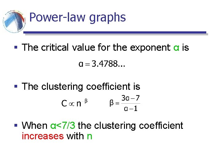
Power-law graphs § The critical value for the exponent α is § The clustering coefficient is § When α<7/3 the clustering coefficient increases with n

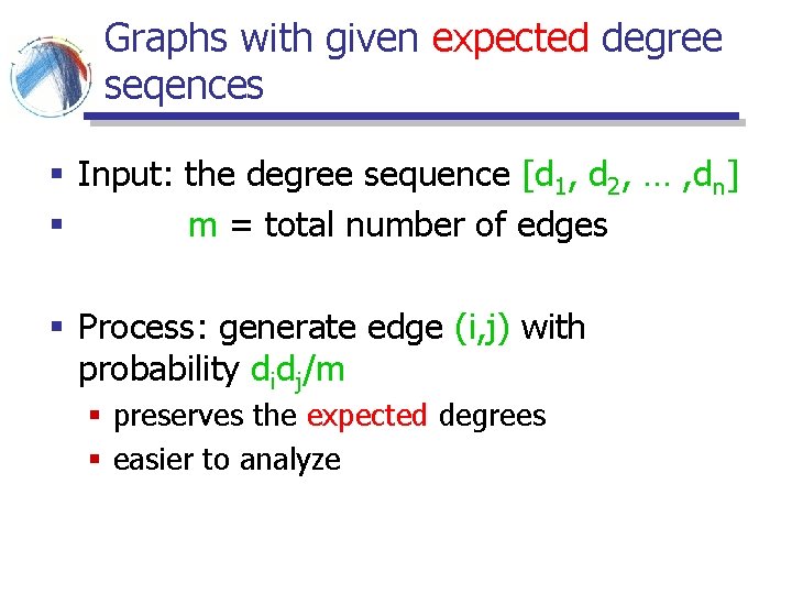
Graphs with given expected degree seqences § Input: the degree sequence [d 1, d 2, … , dn] § m = total number of edges § Process: generate edge (i, j) with probability didj/m § preserves the expected degrees § easier to analyze

However… § The problem is that these models are too contrived § It would be more interesting if the network structure emerged as a side product of a stochastic process rather than fixing its properties in advance.

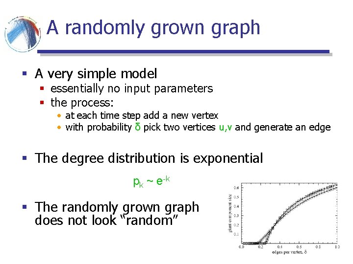
A randomly grown graph § A very simple model § essentially no input parameters § the process: • at each time step add a new vertex • with probability δ pick two vertices u, v and generate an edge § The degree distribution is exponential pk ~ e-k § The randomly grown graph does not look “random”

Preferential Attachment in Networks § First considered by [Price 65] as a model for citation networks § each new paper is generated with m citations (mean) § new papers cite previous papers with probability proportional to their indegree (citations) § what about papers without any citations? • each paper is considered to have a “default” citation • probability of citing a paper with degree k, proportional to k+1 § Power law with exponent α = 2+1/m

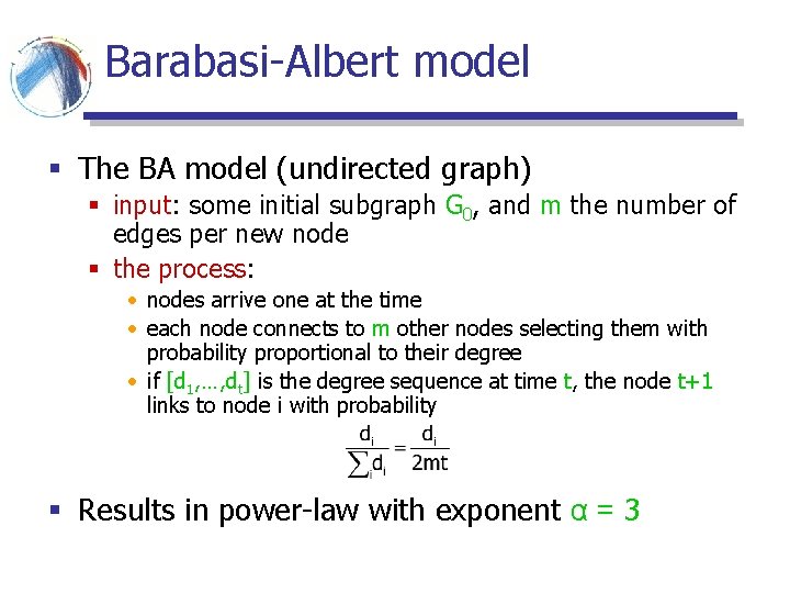
Barabasi-Albert model § The BA model (undirected graph) § input: some initial subgraph G 0, and m the number of edges per new node § the process: • nodes arrive one at the time • each node connects to m other nodes selecting them with probability proportional to their degree • if [d 1, …, dt] is the degree sequence at time t, the node t+1 links to node i with probability § Results in power-law with exponent α = 3

The mathematicians point of view [Bollobas-Riordan] § Self loops and multiple edges are allowed § The m edges are inserted sequentially, thus the problem reduces to studying the single edge problem. § For the single edge problem: § At time t, a new vertex v, connects to an existing vertex u with probability § it creates a self-loop with probability

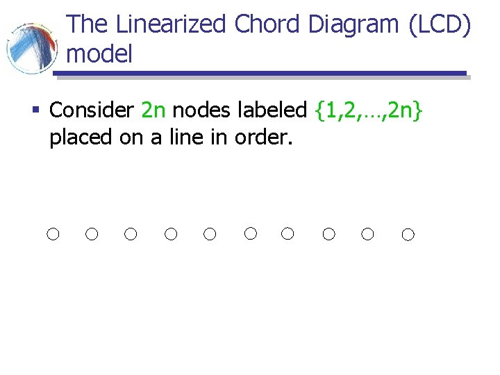
The Linearized Chord Diagram (LCD) model § Consider 2 n nodes labeled {1, 2, …, 2 n} placed on a line in order.

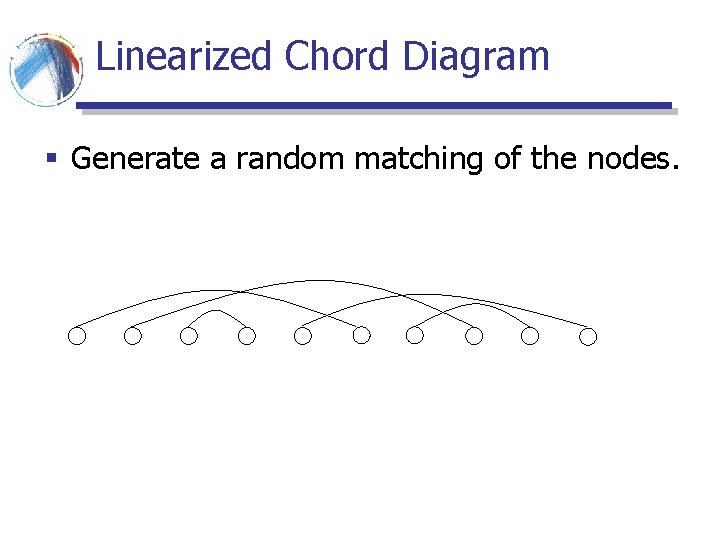
Linearized Chord Diagram § Generate a random matching of the nodes.

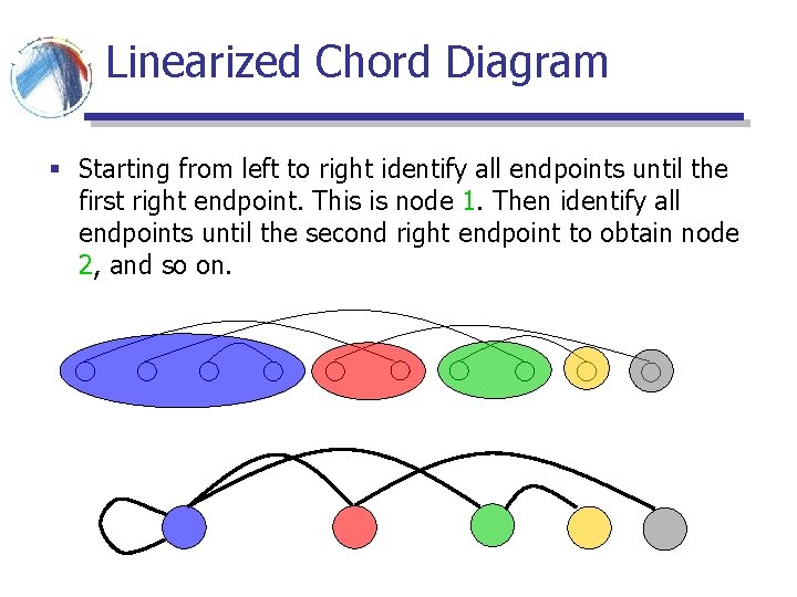
Linearized Chord Diagram § Starting from left to right identify all endpoints until the first right endpoint. This is node 1. Then identify all endpoints until the second right endpoint to obtain node 2, and so on.

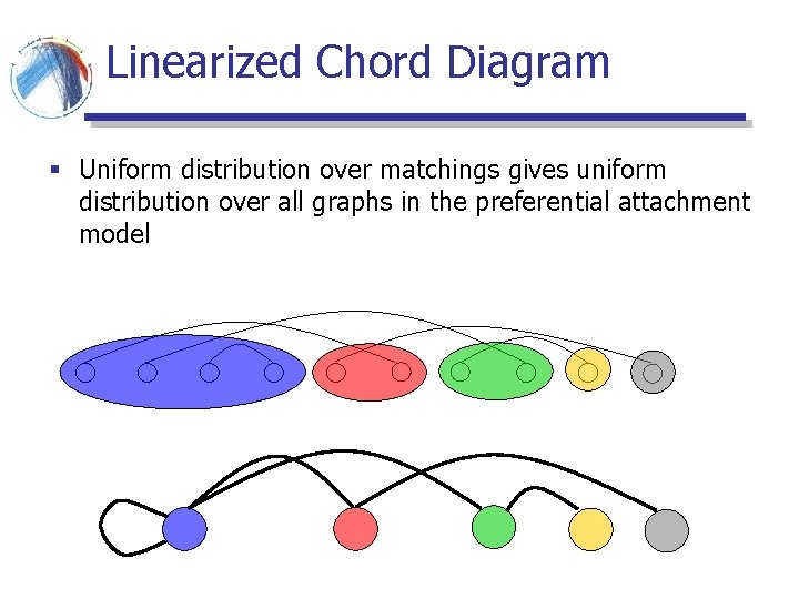
Linearized Chord Diagram § Uniform distribution over matchings gives uniform distribution over all graphs in the preferential attachment model

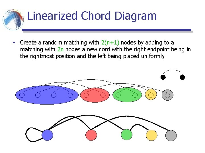
Linearized Chord Diagram § Create a random matching with 2(n+1) nodes by adding to a matching with 2 n nodes a new cord with the right endpoint being in the rightmost position and the left being placed uniformly

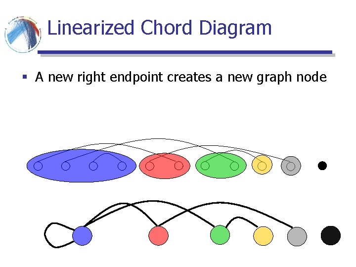
Linearized Chord Diagram § A new right endpoint creates a new graph node

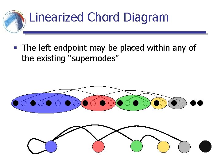
Linearized Chord Diagram § The left endpoint may be placed within any of the existing “supernodes”

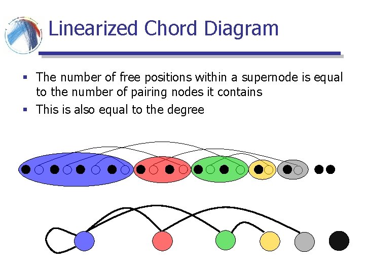
Linearized Chord Diagram § The number of free positions within a supernode is equal to the number of pairing nodes it contains § This is also equal to the degree

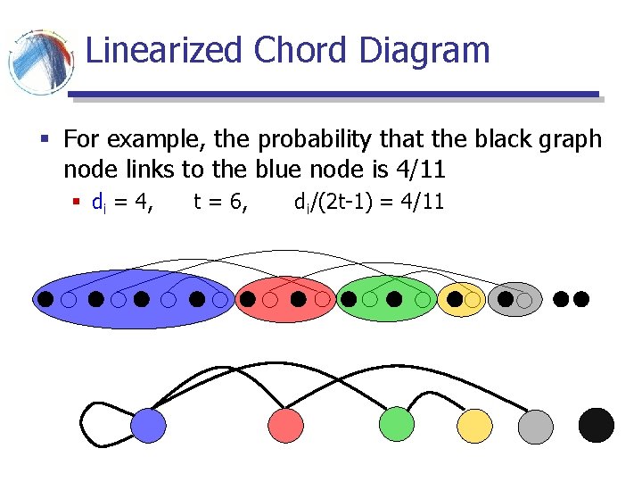
Linearized Chord Diagram § For example, the probability that the black graph node links to the blue node is 4/11 § di = 4, t = 6, di/(2 t-1) = 4/11

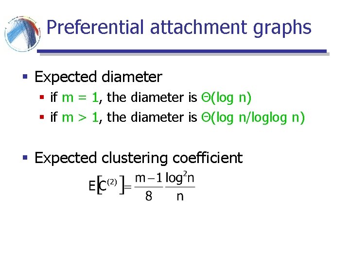
Preferential attachment graphs § Expected diameter § if m = 1, the diameter is Θ(log n) § if m > 1, the diameter is Θ(log n/loglog n) § Expected clustering coefficient

Weaknesses of the BA model § Technical issues: § It is not directed (not good as a model for the Web) and when directed it gives acyclic graphs § It focuses mainly on the (in-) degree and does not take into account other parameters (out-degree distribution, components, clustering coefficient) § It correlates age with degree which is not always the case § Academic issues § the model rediscovers the wheel § preferential attachment is not the answer to every power-law § what does “scale-free” mean exactly? § Yet, it was a breakthrough in the network research, that popularized the area

Variations of the BA model § Many variations have been considered some in order to address the problems with the vanilla BA model § § edge rewiring, appearance and disappearance fitness parameters variable mean degree non-linear preferential attachment • surprisingly, only linear preferential attachment yields power-law graphs

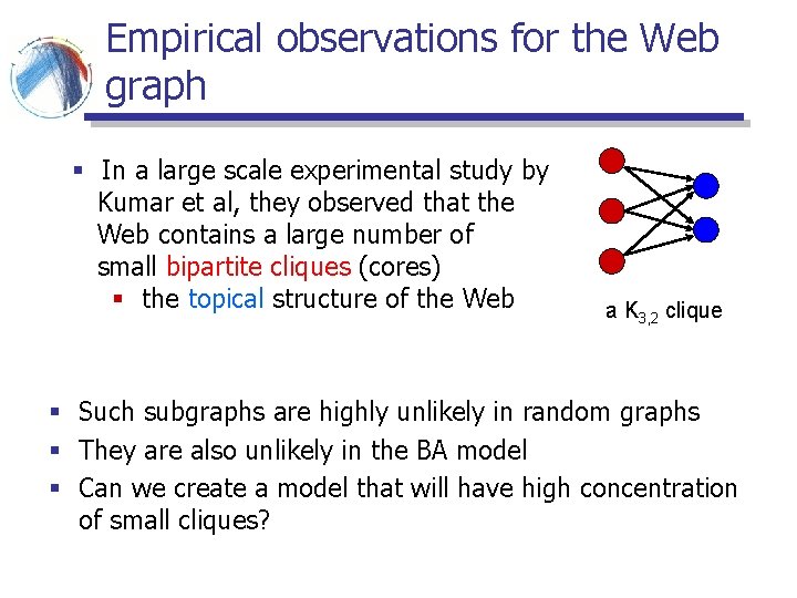
Empirical observations for the Web graph § In a large scale experimental study by Kumar et al, they observed that the Web contains a large number of small bipartite cliques (cores) § the topical structure of the Web a K 3, 2 clique § Such subgraphs are highly unlikely in random graphs § They are also unlikely in the BA model § Can we create a model that will have high concentration of small cliques?

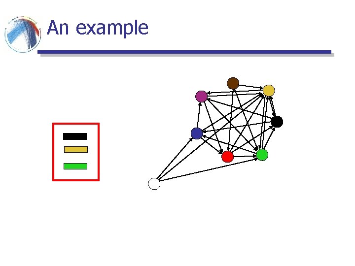
Copying model § Input: § the out-degree d (constant) of each node § a parameter α § The process: § Nodes arrive one at the time § A new node selects uniformly one of the existing nodes as a prototype § The new node creates d outgoing links. For the ith link • with probability α it copies the i-th link of the prototype node • with probability 1 - α it selects the target of the link uniformly at random

An example

Copying model properties § Power law degree distribution with exponent β = (2 -α)/(1 - α) § Number of bipartite cliques of size i x d is ne-i § The model has also found applications in biological networks § copying mechanism in gene mutations

Other graph models § Cooper Frieze model § multiple parameters that allow for adding vertices, edges, preferential attachment, uniform linking § Directed graphs [Bollobas et al] § allow for preferential selection of both the source and the destination § allow for edges from both new and old vertices

Small world Phenomena § So far we focused on obtaining graphs with power-law distributions on the degrees. What about other properties? § Clustering coefficient: real-life networks tend to have high clustering coefficient § Short paths: real-life networks are “small worlds” • this property is easy to generate § Can we combine these two properties?

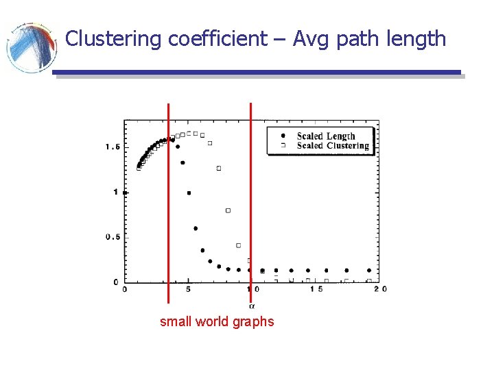
Small-world Graphs § According to Watts [W 99] Large networks (n >> 1) Sparse connectivity (avg degree z << n) No central node (kmax << n) Large clustering coefficient (larger than in random graphs of same size) § Short average paths (~log n, close to those of random graphs of the same size) § §

The Caveman Model [W 99] § The random graph § edges are generated completely at random § low avg. path length L ≤ logn/logz § low clustering coefficient C ~ z/n § The Caveman model § edges follow a structure § high avg. path length L ~ n/z § high clustering coefficient C ~ 1 -O(1/z) § Can we interpolate between the two?

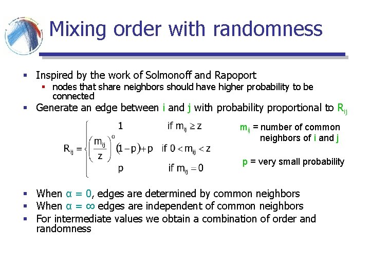
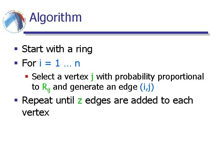
Mixing order with randomness § Inspired by the work of Solmonoff and Rapoport § nodes that share neighbors should have higher probability to be connected § Generate an edge between i and j with probability proportional to Rij mij = number of common neighbors of i and j p = very small probability § When α = 0, edges are determined by common neighbors § When α = ∞ edges are independent of common neighbors § For intermediate values we obtain a combination of order and randomness

Algorithm § Start with a ring § For i = 1 … n § Select a vertex j with probability proportional to Rij and generate an edge (i, j) § Repeat until z edges are added to each vertex

Clustering coefficient – Avg path length small world graphs

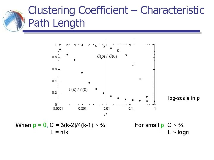
Watts and Strogatz model [WS 98] § Start with a ring, where every node is connected to the next z nodes § With probability p, rewire every edge (or, add a shortcut) to a uniformly chosen destination. § Granovetter, “The strength of weak ties” order p=0 randomness 0<p<1 p=1

Clustering Coefficient – Characteristic Path Length log-scale in p When p = 0, C = 3(k-2)/4(k-1) ~ ¾ L = n/k For small p, C ~ ¾ L ~ logn

Graph Theory Results § Graph theorist failed to be impressed. Most of these results were known.

Evolution of graphs § So far we looked at the properties of graph snapshots. What if we have the history of a graph? § e. g. , citation networks, internet graphs

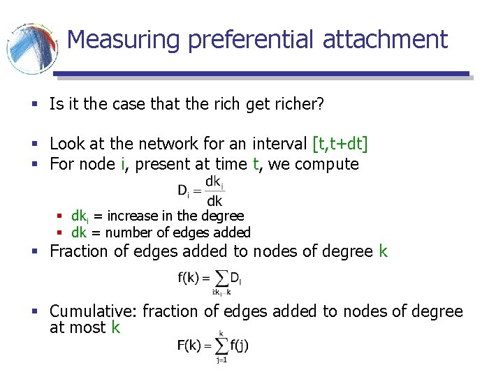
Measuring preferential attachment § Is it the case that the rich get richer? § Look at the network for an interval [t, t+dt] § For node i, present at time t, we compute § dki = increase in the degree § dk = number of edges added § Fraction of edges added to nodes of degree k § Cumulative: fraction of edges added to nodes of degree at most k

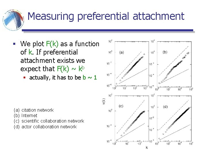
Measuring preferential attachment § We plot F(k) as a function of k. If preferential attachment exists we expect that F(k) ~ kb § actually, it has to be b ~ 1 (a) (b) (c) (d) citation network Internet scientific collaboration network actor collaboration network

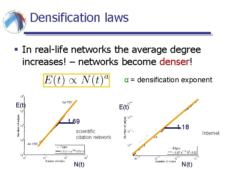
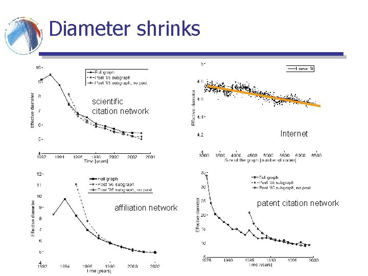
Network models and temporal evolution § For most of the existing models it is assumed that § number of edges grows linearly with the number of nodes § the diameter grows at rate logn, or loglogn § What about real graphs? § Leskovec, Kleinberg, Faloutsos 2005

Densification laws § In real-life networks the average degree increases! – networks become denser! α = densification exponent E(t) 1. 69 scientific citation network N(t) 1. 18 N(t) Internet

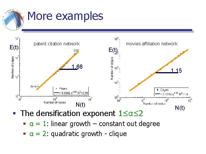
More examples E(t) patent citation network movies affiliation network E(t) 1. 66 N(t) § The densification exponent 1≤α≤ 2 § α = 1: linear growth – constant out degree § α = 2: quadratic growth - clique 1. 15 N(t)

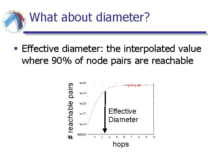
What about diameter? # reachable pairs § Effective diameter: the interpolated value where 90% of node pairs are reachable Effective Diameter hops

Diameter shrinks scientific citation network Internet affiliation network patent citation network

Densification – Possible Explanation § Existing graph generation models do not capture the Densification Power Law and Shrinking diameters § Can we find a simple model of local behavior, which naturally leads to observed phenomena? § Two proposed models § Community Guided Attachment – obeys Densification § Forest Fire model – obeys Densification, Shrinking diameter (and Power Law degree distribution)

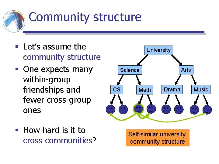
Community structure § Let’s assume the community structure § One expects many within-group friendships and fewer cross-group ones § How hard is it to cross communities? University Arts Science CS Math Drama Self-similar university community structure Music

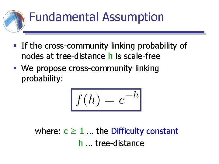
Fundamental Assumption § If the cross-community linking probability of nodes at tree-distance h is scale-free § We propose cross-community linking probability: where: c ≥ 1 … the Difficulty constant h … tree-distance

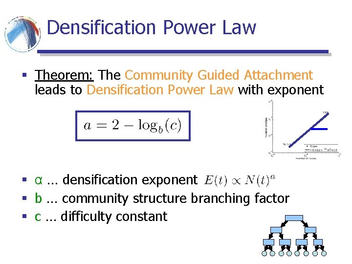
Densification Power Law § Theorem: The Community Guided Attachment leads to Densification Power Law with exponent § α … densification exponent § b … community structure branching factor § c … difficulty constant

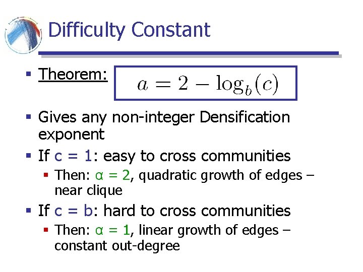
Difficulty Constant § Theorem: § Gives any non-integer Densification exponent § If c = 1: easy to cross communities § Then: α = 2, quadratic growth of edges – near clique § If c = b: hard to cross communities § Then: α = 1, linear growth of edges – constant out-degree

Room for Improvement § Community Guided Attachment explains Densification Power Law § Issues: § Requires explicit Community structure § Does not obey Shrinking Diameters § The ”Forrest Fire” model

“Forest Fire” model – Wish List § We want: § no explicit Community structure § Shrinking diameters § and: • “Rich get richer” attachment process, to get heavytailed in-degrees • “Copying” model, to lead to communities • Community Guided Attachment, to produce Densification Power Law

“Forest Fire” model – Intuition § How do authors identify references? 1. 2. 3. 4. Find first paper and cite it Follow a few citations, make citations Continue recursively From time to time use bibliographic tools (e. g. Cite. Seer) and chase back-links

“Forest Fire” model – Intuition § How do people make friends in a new environment? 1. Find first a person and make friends 2. From time to time get introduced to his friends 3. Continue recursively § Forest Fire model imitates exactly this process

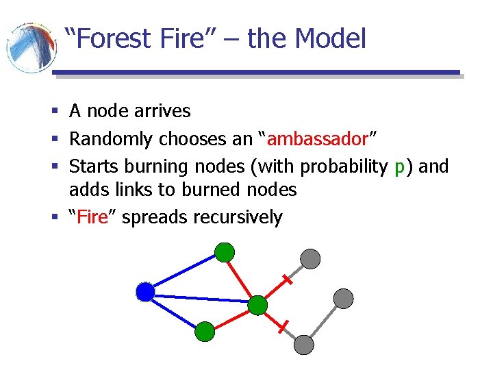
“Forest Fire” – the Model § A node arrives § Randomly chooses an “ambassador” § Starts burning nodes (with probability p) and adds links to burned nodes § “Fire” spreads recursively

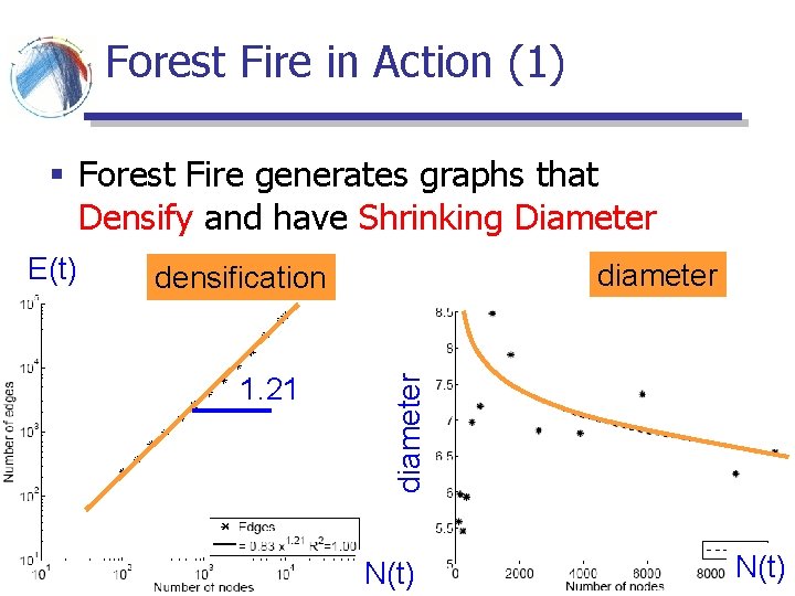
Forest Fire in Action (1) § Forest Fire generates graphs that Densify and have Shrinking Diameter densification 1. 21 diameter E(t) N(t)

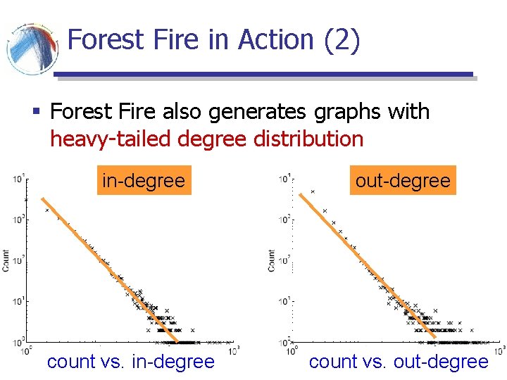
Forest Fire in Action (2) § Forest Fire also generates graphs with heavy-tailed degree distribution in-degree count vs. in-degree out-degree count vs. out-degree

Forest Fire model – Justification § Densification Power Law: § Similar to Community Guided Attachment § The probability of linking decays exponentially with the distance – Densification Power Law § Power law out-degrees: § From time to time we get large fires § Power law in-degrees: § The fire is more likely to reach hubs

Forest Fire model – Justification § Communities: § Newcomer copies neighbors’ links § Shrinking diameter

Acknowledgements § Many thanks to Jure Leskovec for his slides from the KDD 2005 paper.

References § M. E. J. Newman, The structure and function of complex networks, SIAM Reviews, 45(2): 167 -256, 2003 § R. Albert and L. A. Barabasi, Statistical Mechanics of Complex Networks, Rev. Mod. Phys. 74, 47 -97 (2002). § B. Bollobas, Mathematical Results in Scale-Free random Graphs § D. J. Watts. Networks, Dynamics and Small-World Phenomenon, American Journal of Sociology, Vol. 105, Number 2, 493 -527, 1999 § Watts, D. J. and S. H. Strogatz. Collective dynamics of 'small-world' networks. Nature 393: 440 -42, 1998 § D. Callaway, J. Hopcroft, J. Kleinberg, M. Newman, S. Strogatz. Are randomly grown graphs really random? Physical Review E 64, 041902 (2001). § J. Leskovec, J. Kleinberg, C. Faloutsos. Graphs over Time: Densification Laws, Shrinking Diameters and Possible Explanations. Proc. 11 th ACM SIGKDD Intl. Conf. on Knowledge Discovery and Data Mining, 2005.