Modelling Simulation of Semiconductor Devices Lecture 1 2

Modelling & Simulation of Semiconductor Devices Lecture 1 & 2 Introduction to Modelling & Simulation

Systems • What is System? – Components – relationship – objective 2

Systems • What is System – A system is a set of components which are related by some form of interaction and which act together to achieve some objective or purpose • Components are the individual parts or elements that collectively make up the system • Relationships are the cause-effect dependencies between components • Objective is the desired state or outcome which the system is attempting to achieve 3

Types of Systems • • Static System: If a system does not change with time, it is called a static system. Dynamic System: If a system changes with time, it is called a dynamic system. 4

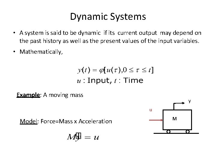
Dynamic Systems • A system is said to be dynamic if its current output may depend on the past history as well as the present values of the input variables. • Mathematically, Example: A moving mass y u Model: Force=Mass x Acceleration M

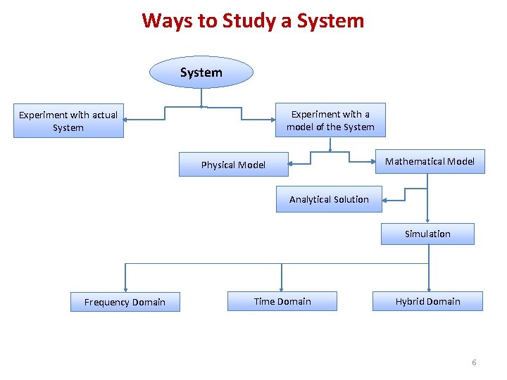
Ways to Study a System Experiment with a model of the System Experiment with actual System Mathematical Model Physical Model Analytical Solution Simulation Frequency Domain Time Domain Hybrid Domain 6

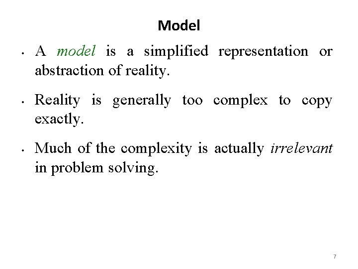
Model • • • A model is a simplified representation or abstraction of reality. Reality is generally too complex to copy exactly. Much of the complexity is actually irrelevant in problem solving. 7

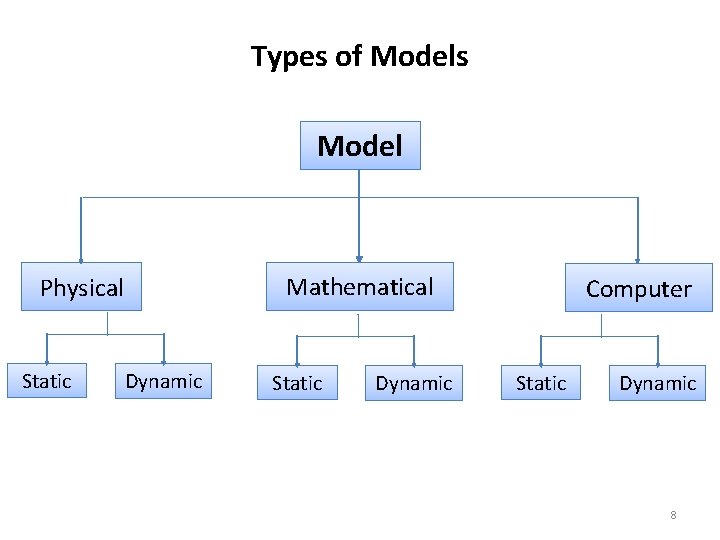
Types of Models Model Mathematical Physical Static Dynamic Computer Static Dynamic 8

What is Mathematical Model? A set of mathematical equations (e. g. , differential eqs. ) that describes the input-output behavior of a system. What is a model used for? • Simulation • Prediction/Forecasting • Prognostics/Diagnostics • Design/Performance Evaluation • Control System Design

Classification of Mathematical Models • Linear vs. Non-linear • Deterministic vs. Probabilistic (Stochastic) • Static vs. Dynamic • Discrete vs. Continuous • White box, black box and gray box 10

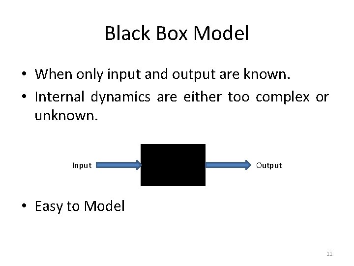
Black Box Model • When only input and output are known. • Internal dynamics are either too complex or unknown. Input Output • Easy to Model 11

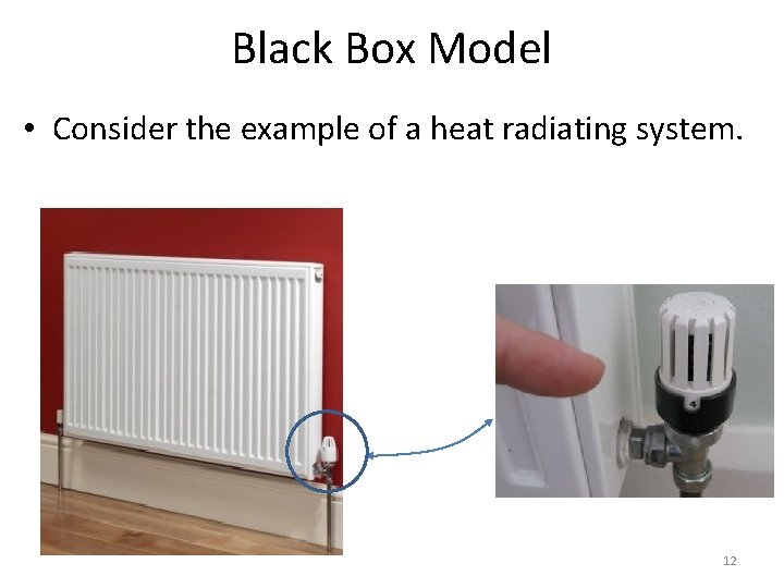
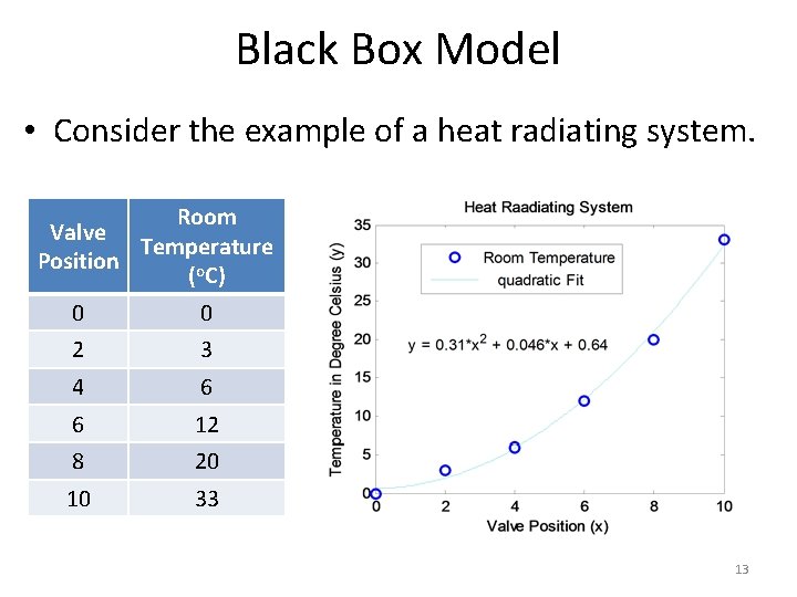
Black Box Model • Consider the example of a heat radiating system. 12

Black Box Model • Consider the example of a heat radiating system. Room Valve Temperature Position (o. C) 0 0 2 3 4 6 6 12 8 20 10 33 13

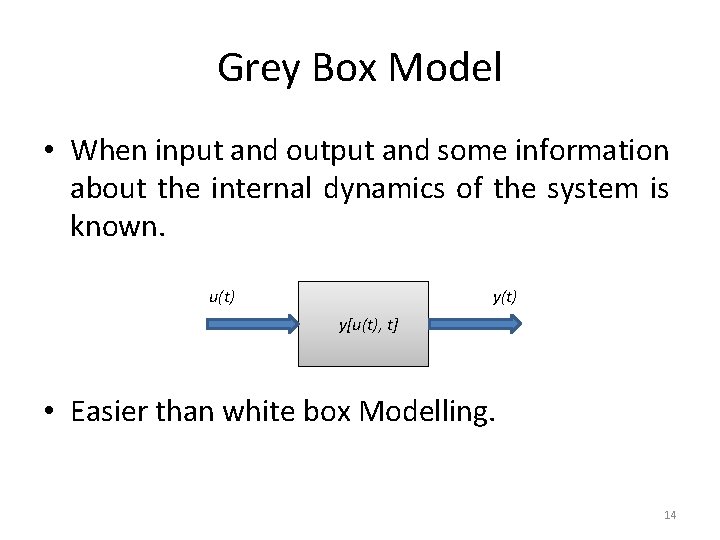
Grey Box Model • When input and output and some information about the internal dynamics of the system is known. u(t) y[u(t), t] • Easier than white box Modelling. 14

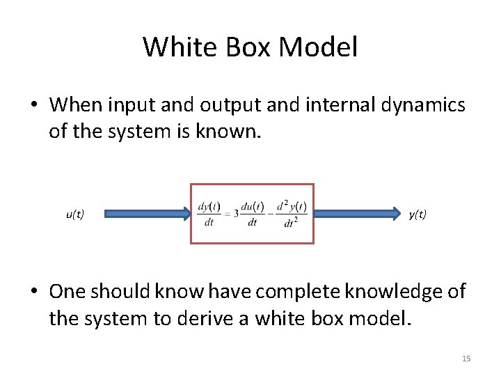
White Box Model • When input and output and internal dynamics of the system is known. u(t) y(t) • One should know have complete knowledge of the system to derive a white box model. 15

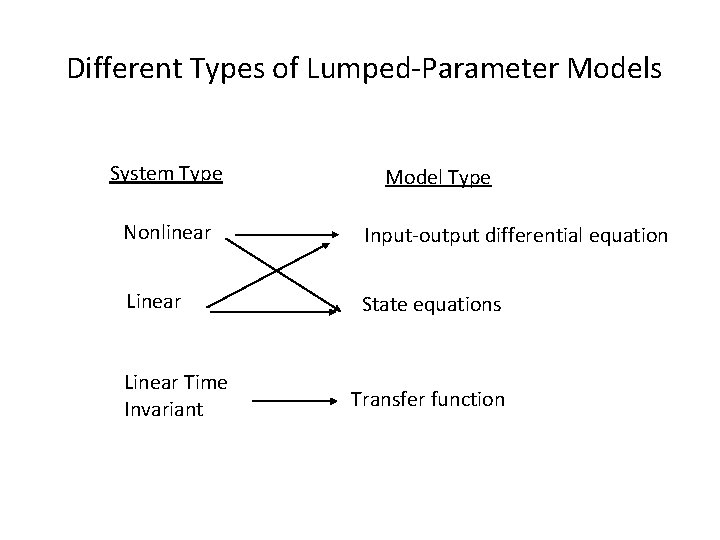
Mathematical Modelling Basics Mathematical model of a real world system is derived using a combination of physical laws and/or experimental means • Physical laws are used to determine the model structure (linear or nonlinear) and order. • The parameters of the model are often estimated and/or validated experimentally. • Mathematical model of a dynamic system can often be expressed as a system of differential (difference in the case of discrete-time systems) equations

Different Types of Lumped-Parameter Models System Type Model Type Nonlinear Input-output differential equation Linear State equations Linear Time Invariant Transfer function

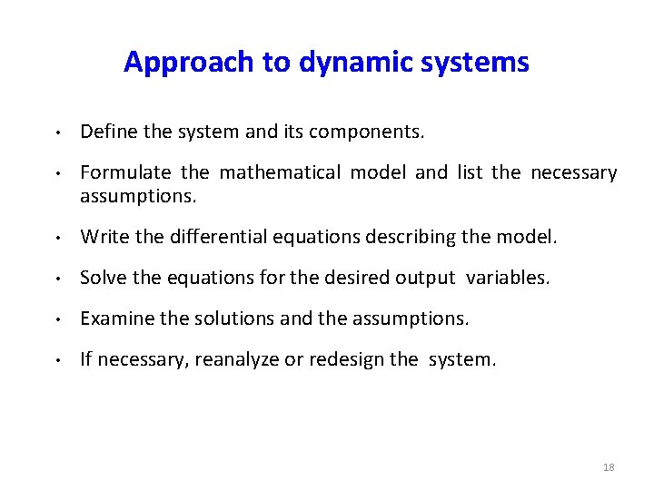
Approach to dynamic systems • Define the system and its components. • Formulate the mathematical model and list the necessary assumptions. • Write the differential equations describing the model. • Solve the equations for the desired output variables. • Examine the solutions and the assumptions. • If necessary, reanalyze or redesign the system. 18

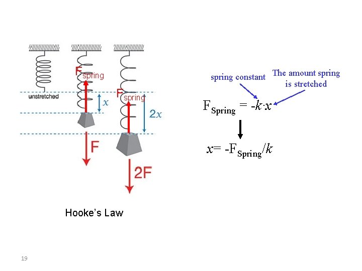
Fspring constant The amount spring is stretched FSpring = -k∙x x= -FSpring/k Hooke’s Law 19

Simulation • • Computer simulation is the discipline of designing a model of an actual or theoretical physical system, executing the model on a digital computer, and analyzing the execution output. Simulation embodies the principle of ``learning by doing'' --- to learn about the system we must first build a model of some sort and then operate the model. 20

Advantages to Simulation q q Can be used to study existing systems without disrupting the ongoing operations. Proposed systems can be “tested” before committing resources. Allows us to control time. Allows us to gain insight into which variables are most important to system performance. 21

Disadvantages to Simulation q q Model building is an art as well as a science. The quality of the analysis depends on the quality of the model and the skill of the modeler. Simulation results are sometimes hard to interpret. Simulation analysis can be time consuming and expensive. Should not be used when an analytical method would provide for quicker results. 22

Model Development: A case study LECTURE – II

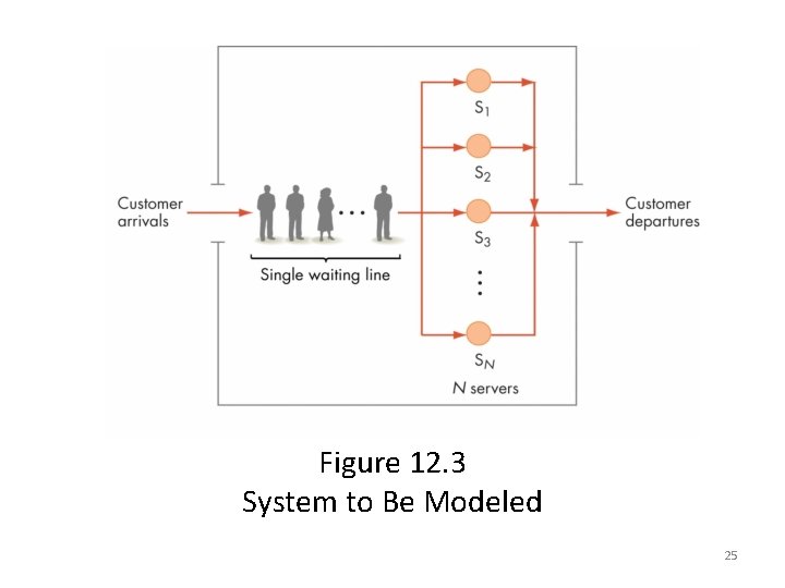
An Example of Model Building (continued) – You are the owner of a new take-out restaurant, Mc. Burgers, currently under construction – You want to determine the proper number of checkout stations needed – You decide to build a model of Mc. Burgers to determine the optimal number of servers 24 • Problem

Figure 12. 3 System to Be Modeled 25

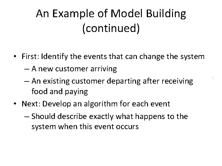
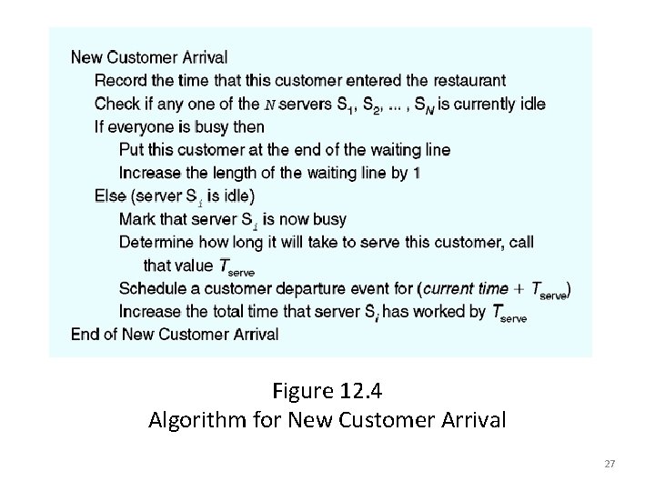
• First: Identify the events that can change the system – A new customer arriving – An existing customer departing after receiving food and paying • Next: Develop an algorithm for each event – Should describe exactly what happens to the system when this event occurs 26 An Example of Model Building (continued)

Figure 12. 4 Algorithm for New Customer Arrival 27

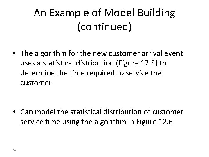
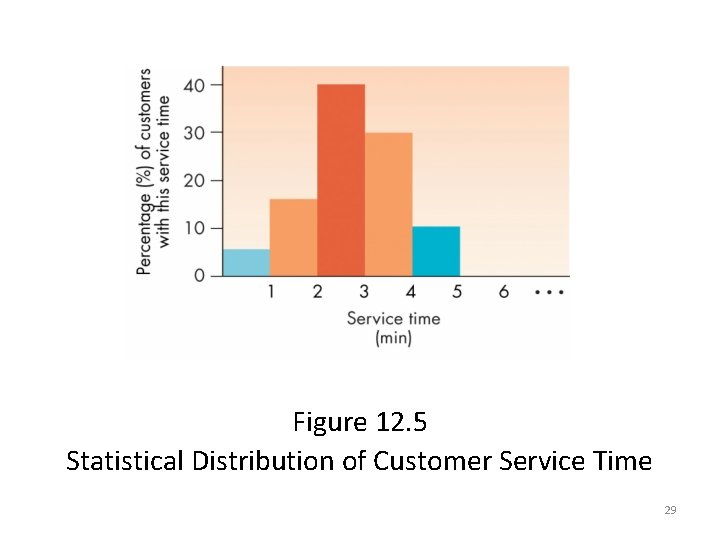
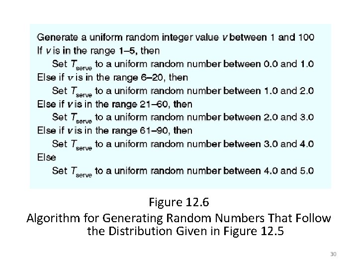
An Example of Model Building (continued) • The algorithm for the new customer arrival event uses a statistical distribution (Figure 12. 5) to determine the time required to service the customer • Can model the statistical distribution of customer service time using the algorithm in Figure 12. 6 28

Figure 12. 5 Statistical Distribution of Customer Service Time 29

Figure 12. 6 Algorithm for Generating Random Numbers That Follow the Distribution Given in Figure 12. 5 30

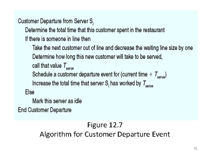
Figure 12. 7 Algorithm for Customer Departure Event 31

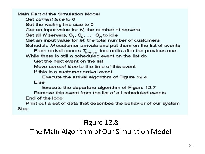
An Example of Model Building (continued) • Must initialize parameters to the model • Model must collect data that accurately measures performance of the Mc. Burgers restaurant 32

An Example of Model Building (continued) • When simulation is ready, the computer will – Run the simulation – Process all M customers – Print out the results 33

Figure 12. 8 The Main Algorithm of Our Simulation Model 34

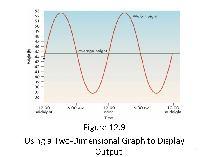
Running the Model and Visualizing Results • Scientific visualization – Visualizing data in a way that highlights important characteristics and simplifies its interpretation – An important part of computational modeling – Different from computer graphics 35

Running the Model and Visualizing Results (continued) • Scientific visualization is concerned with – Data extraction: Determine which data values are important to display and which are not – Data manipulation: Convert the data to other forms or to different units to enhance display 36

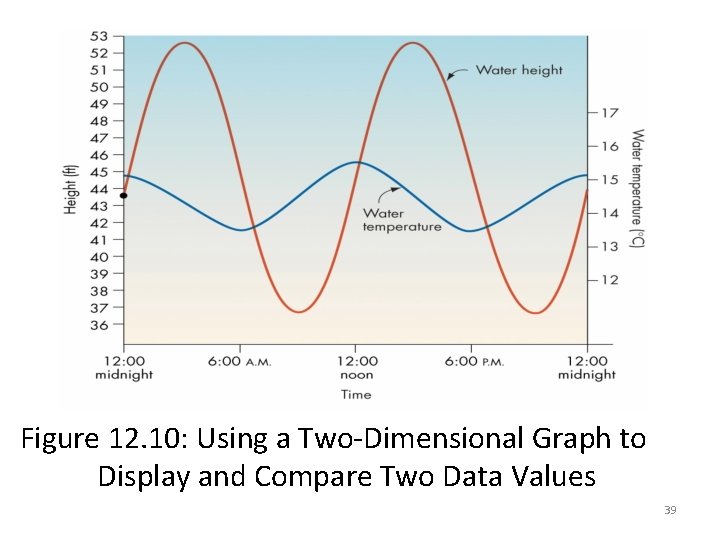
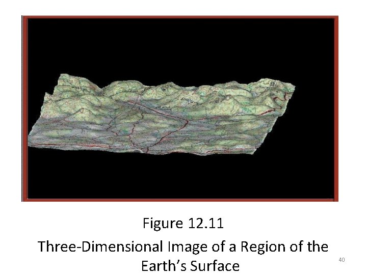
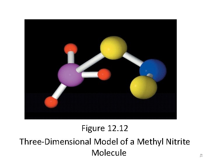
Running the Model and Visualizing Results (continued) • Output of a computer model can be represented visually using – A two-dimensional graph – A three-dimensional image • Visual representation of data helps identify important features of the model’s output 37

Figure 12. 9 Using a Two-Dimensional Graph to Display Output 38

Figure 12. 10: Using a Two-Dimensional Graph to Display and Compare Two Data Values 39

Figure 12. 11 Three-Dimensional Image of a Region of the Earth’s Surface 40

41 Figure 12. 12 Three-Dimensional Model of a Methyl Nitrite Molecule

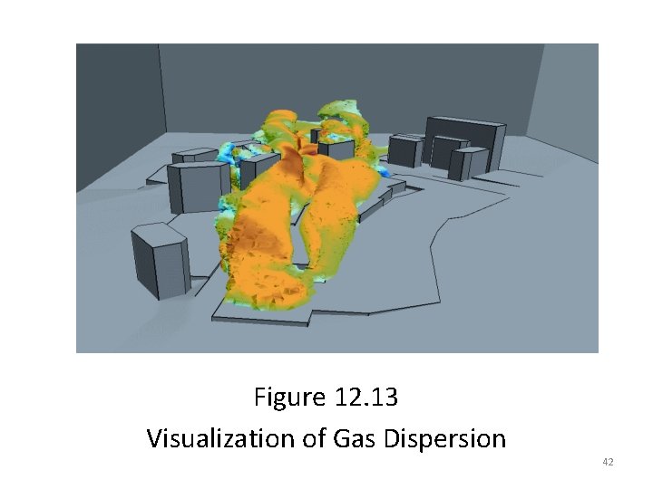
Figure 12. 13 Visualization of Gas Dispersion 42

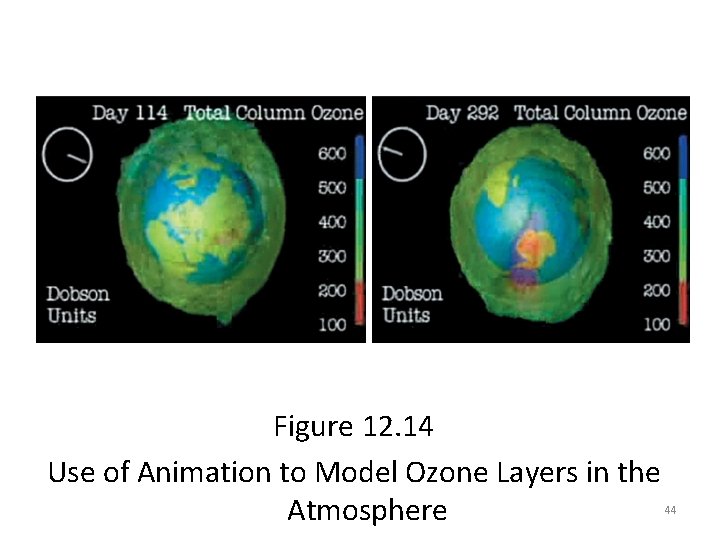
Running the Model and Visualizing Results (continued) – One of the most powerful and useful forms of visualization – Shows how model’s output changes over time – Created using many images, each showing system state at a slightly later point in time 43 • Image animation

Figure 12. 14 Use of Animation to Model Ozone Layers in the Atmosphere 44

To download this lecture visit http: //imtiazhussainkalwar. weebly. com/ END OF LECTURES 1 -2 45