Modelling of Energy Systems Renewables and Efficiency Rangan

Modelling of Energy Systems. Renewables and Efficiency Rangan Banerjee Department of Energy Science and Engineering IIT Bombay Seminar at Strathclyde University, June 2, 2009

Indian Examples n n n Analysis of wind integration into power system PV- Battery storage – Design space Solar Water Heater Diffusion Optimal response to time of use tariff - process scheduling - cool storage -cogeneration Benchmarking of glass furnace Decision Support System for energy planning

Issues in grid integration n n Conventional power planning- hydrothermal scheduling How do we deal with renewables? Capacity credit New methodology based on Load Duration Curve Illustrated for Wind in Tamil Nadu

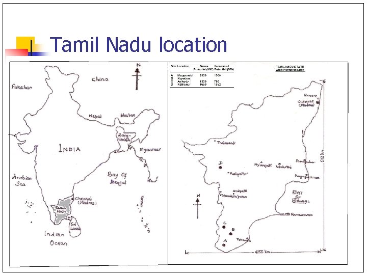
Tamil Nadu location

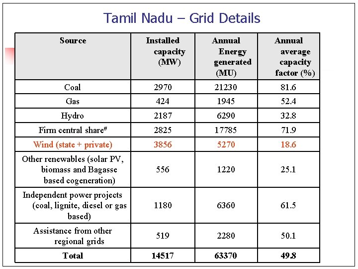
Tamil Nadu – Grid Details Source Installed capacity (MW) Annual Energy generated (MU) Annual average capacity factor (%) Coal 2970 21230 81. 6 Gas 424 1945 52. 4 Hydro 2187 6290 32. 8 Firm central share 2825 17785 71. 9 Wind (state + private) 3856 5270 18. 6 Other renewables (solar PV, biomass and Bagasse based cogeneration) 556 1220 25. 1 Independent power projects (coal, lignite, diesel or gas based) 1180 6360 61. 5 Assistance from other regional grids 519 2280 50. 1 Total 14517 63370 49. 8

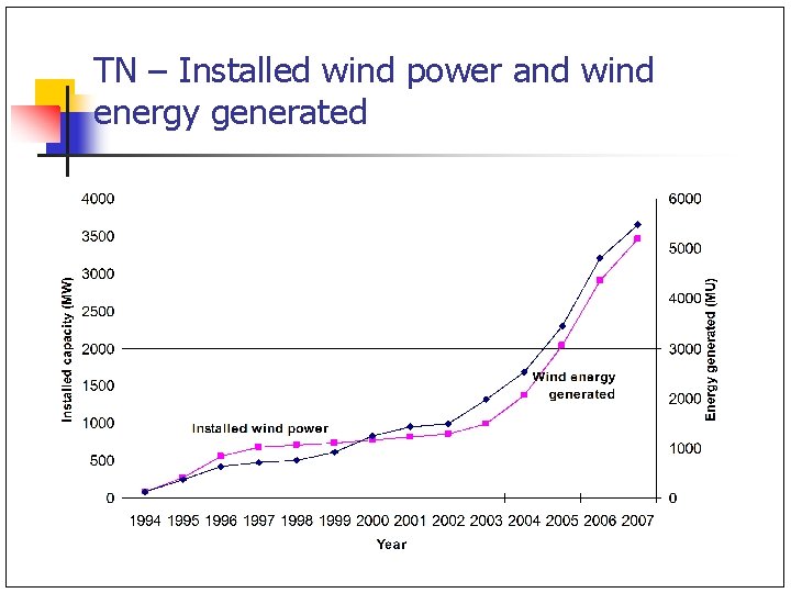
TN – Installed wind power and wind energy generated

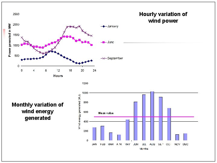
Hourly variation of wind power Monthly variation of wind energy generated

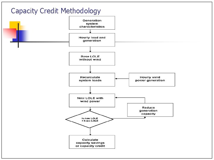
Capacity Credit Methodology

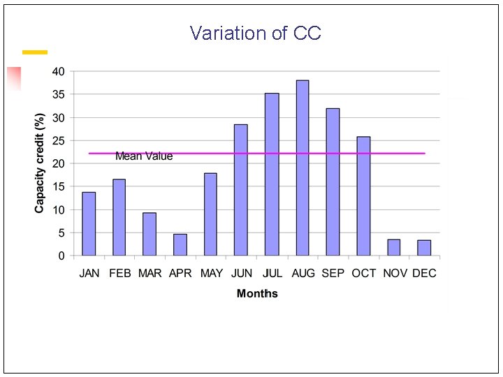
Variation of CC

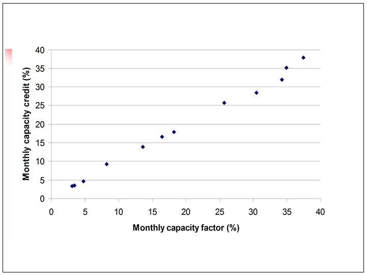
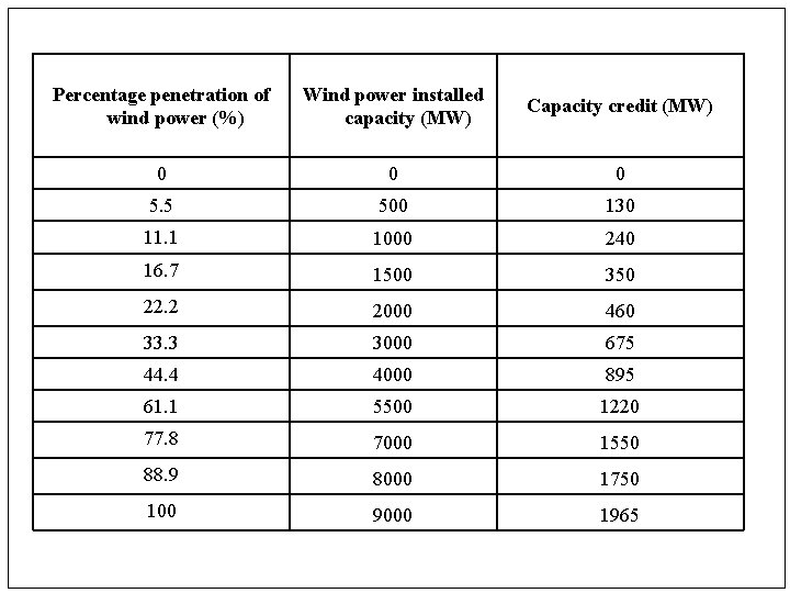
Percentage penetration of wind power (%) Wind power installed capacity (MW) Capacity credit (MW) 0 0 0 5. 5 500 130 11. 1 1000 240 16. 7 1500 350 22. 2 2000 460 33. 3 3000 675 44. 4 4000 895 61. 1 5500 1220 77. 8 7000 1550 88. 9 8000 1750 100 9000 1965

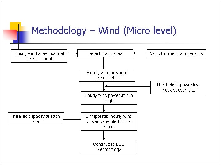
Methodology – Wind (Micro level) Hourly wind speed data at sensor height Select major sites Wind turbine characteristics Hourly wind power at sensor height Hub height, power law index at each site Hourly wind power at hub height Installed capacity at each site Extrapolated hourly wind power generated in the state Continue to LDC Methodology

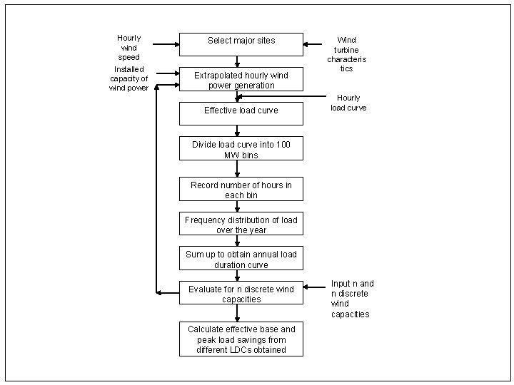
Hourly wind speed data Installed capacity of wind power Select major sites Extrapolated hourly wind power generation Effective load curve Wind turbine characteris tics Hourly load curve Divide load curve into 100 MW bins Record number of hours in each bin Frequency distribution of load over the year Sum up to obtain annual load duration curve Evaluate for n discrete wind capacities Calculate effective base and peak load savings from different LDCs obtained Input n and n discrete wind capacities

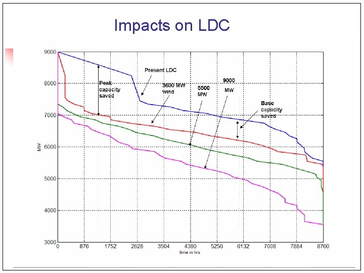
Impacts on LDC

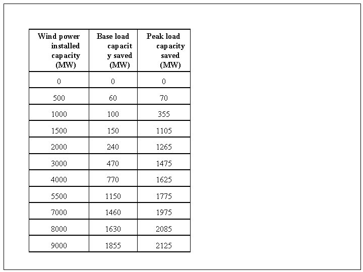
Wind power installed capacity (MW) Base load capacit y saved (MW) Peak load capacity saved (MW) 0 0 0 500 60 70 100 355 1500 150 1105 2000 240 1265 3000 470 1475 4000 770 1625 5500 1150 1775 7000 1460 1975 8000 1630 2085 9000 1855 2125

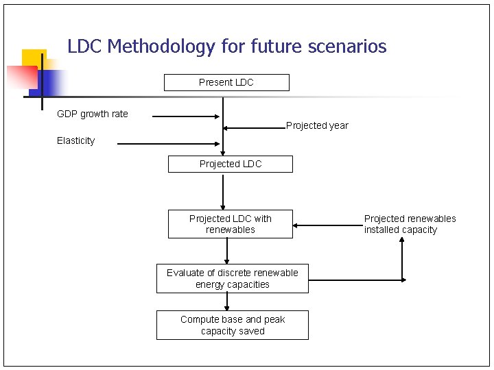
LDC Methodology for future scenarios Present LDC GDP growth rate Projected year Elasticity Projected LDC with renewables Evaluate of discrete renewable energy capacities Compute base and peak capacity saved Projected renewables installed capacity

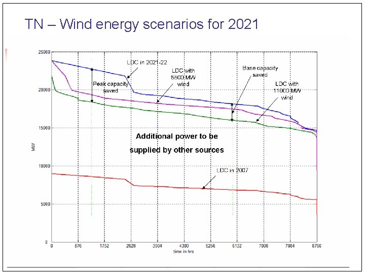
TN – Wind energy scenarios for 2021

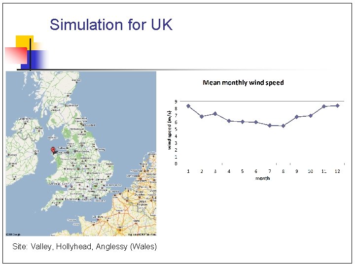
Simulation for UK Site: Valley, Hollyhead, Anglessy (Wales)

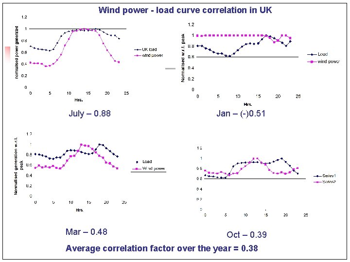
Wind power - load curve correlation in UK July – 0. 88 Mar – 0. 48 Jan – (-)0. 51 Oct – 0. 39 Average correlation factor over the year = 0. 38

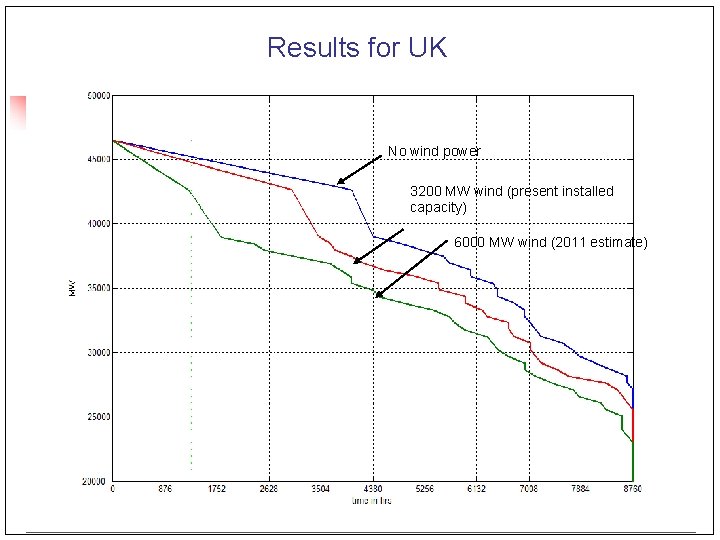
Results for UK No wind power 3200 MW wind (present installed capacity) 6000 MW wind (2011 estimate)

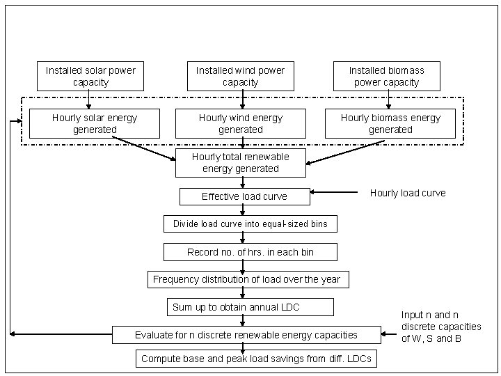
Installed solar power capacity Installed wind power capacity Hourly solar energy generated Hourly wind energy generated Installed biomass power capacity Hourly biomass energy generated Hourly total renewable energy generated Effective load curve Hourly load curve Divide load curve into equal-sized bins Record no. of hrs. in each bin Frequency distribution of load over the year Sum up to obtain annual LDC Evaluate for n discrete renewable energy capacities Compute base and peak load savings from diff. LDCs Input n and n discrete capacities of W, S and B

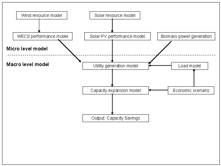
Wind resource model WECS performance model Solar resource model Solar PV performance model Biomass power generation Micro level model Macro level model Utility generation model Load model Capacity expansion model Economic scenario Output: Capacity Savings

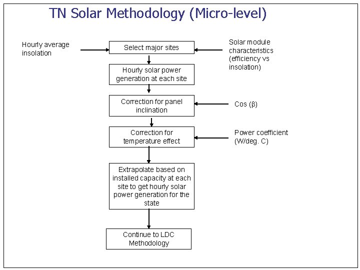
TN Solar Methodology (Micro-level) Hourly average insolation Select major sites Hourly solar power generation at each site Correction for panel inclination Correction for temperature effect Extrapolate based on installed capacity at each site to get hourly solar power generation for the state Continue to LDC Methodology Solar module characteristics (efficiency vs insolation) Cos ( ) Power coefficient (W/deg. C)

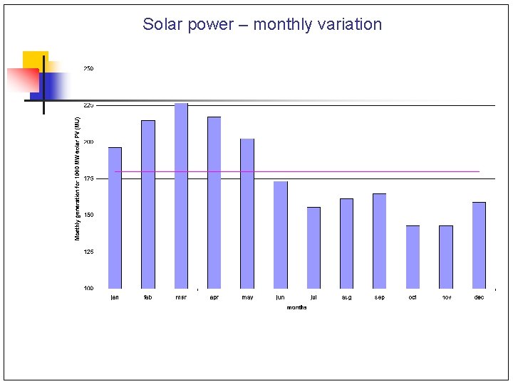
Solar power – monthly variation

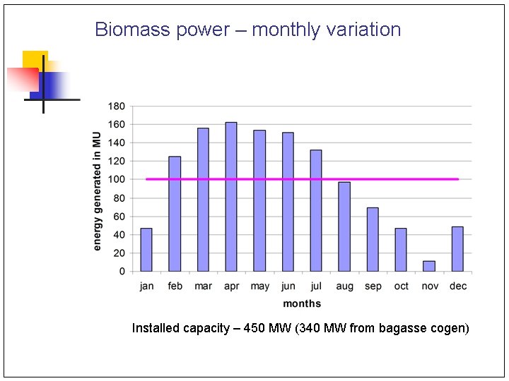
Biomass power – monthly variation Installed capacity – 450 MW (340 MW from bagasse cogen)

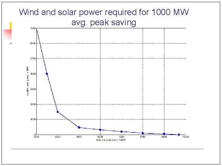
Wind and solar power required for 1000 MW avg. peak saving

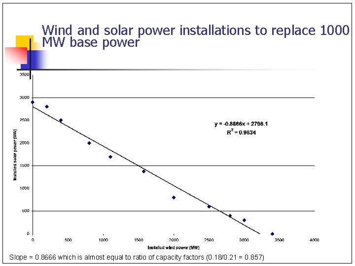
Wind and solar power installations to replace 1000 MW base power Slope = 0. 8666 which is almost equal to ratio of capacity factors (0. 18/0. 21 = 0. 857)

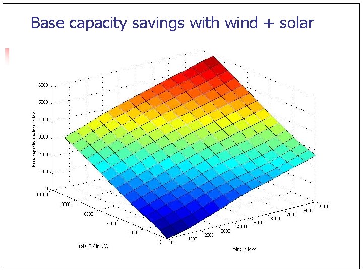
Base capacity savings with wind + solar

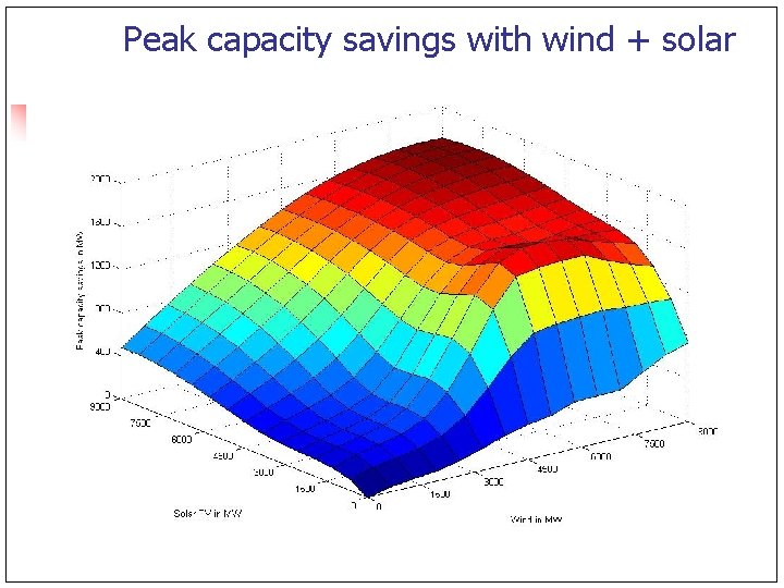
Peak capacity savings with wind + solar

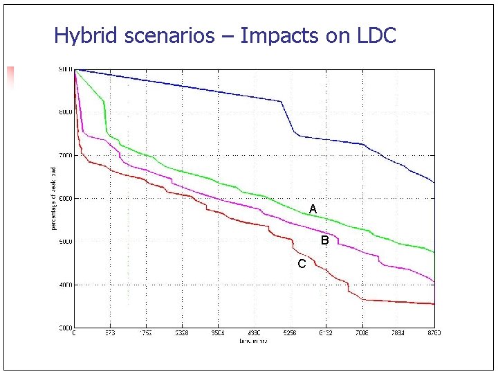
Hybrid scenarios – Impacts on LDC A B C

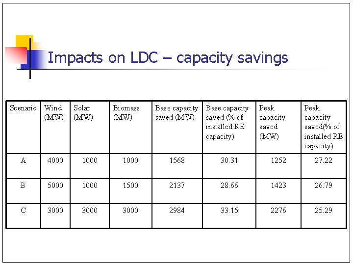
Impacts on LDC – capacity savings Scenario Wind (MW) Solar (MW) Biomass (MW) Base capacity saved (MW) saved (% of installed RE capacity) Peak capacity saved (MW) Peak capacity saved(% of installed RE capacity) A 4000 1000 1568 30. 31 1252 27. 22 B 5000 1500 2137 28. 66 1423 26. 79 C 3000 2984 33. 15 2276 25. 29

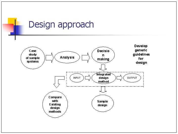
Design approach Case study of sample systems Analysis INPUT Compare with Existing design methods Decisio n making Integrated design method Sample design Develop generic guidelines for design OUTPUT

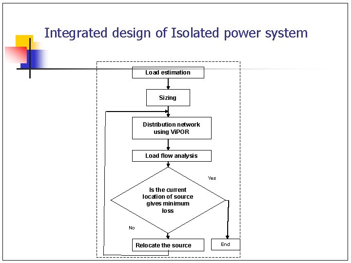
Integrated design of Isolated power system Load estimation Sizing Distribution network using Vi. POR Load flow analysis Yes Is the current location of source gives minimum loss No Relocate the source End

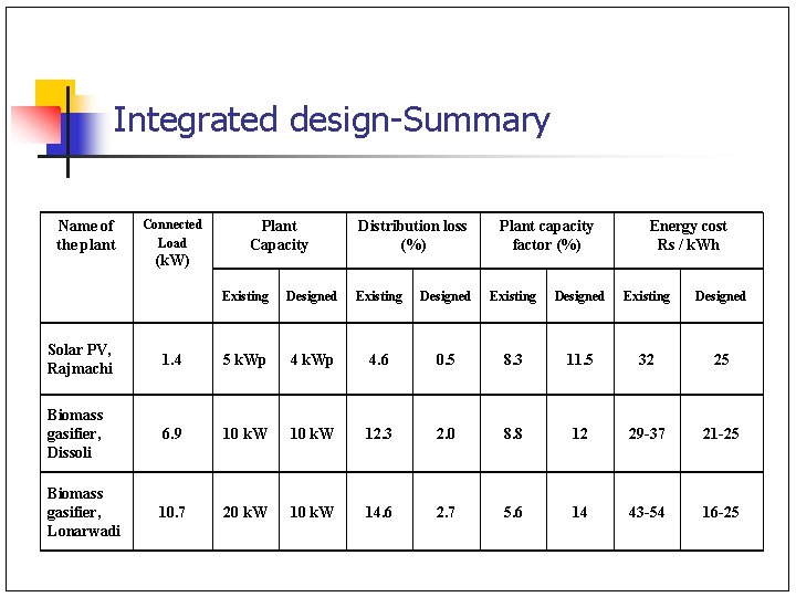
Integrated design-Summary Name of the plant Connected Load (k. W) Plant Capacity Distribution loss (%) Plant capacity factor (%) Energy cost Rs / k. Wh Existing Designed Solar PV, Rajmachi 1. 4 5 k. Wp 4. 6 0. 5 8. 3 11. 5 32 25 Biomass gasifier, Dissoli 6. 9 10 k. W 12. 3 2. 0 8. 8 12 29 -37 21 -25 Biomass gasifier, Lonarwadi 10. 7 20 k. W 14. 6 2. 7 5. 6 14 43 -54 16 -25

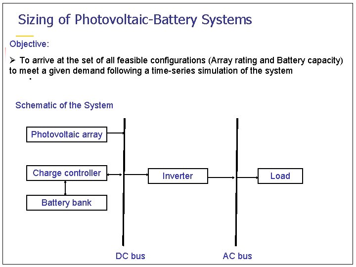
Sizing of Photovoltaic-Battery Systems Objective: Ø To arrive at the set of all feasible configurations (Array rating and Battery capacity) to meet a given demand following a time-series simulation of the system Schematic of the System Photovoltaic array Charge controller Inverter Load Battery bank DC bus AC bus

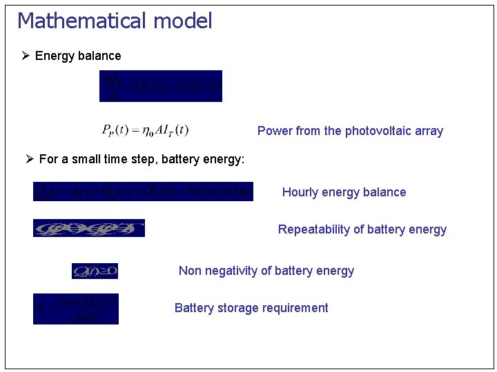
Mathematical model Ø Energy balance Power from the photovoltaic array Ø For a small time step, battery energy: Hourly energy balance Repeatability of battery energy Non negativity of battery energy Battery storage requirement

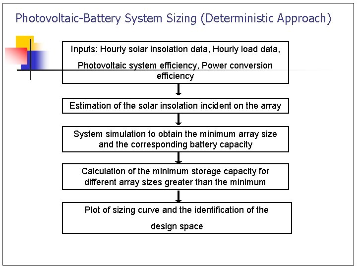
Photovoltaic-Battery System Sizing (Deterministic Approach) Inputs: Hourly solar insolation data, Hourly load data, Photovoltaic system efficiency, Power conversion efficiency Estimation of the solar insolation incident on the array System simulation to obtain the minimum array size and the corresponding battery capacity Calculation of the minimum storage capacity for different array sizes greater than the minimum Plot of sizing curve and the identification of the design space

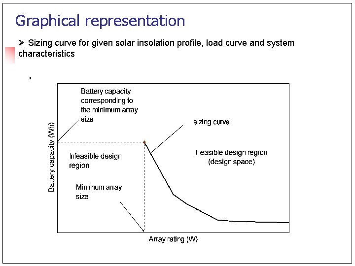
Graphical representation Ø Sizing curve for given solar insolation profile, load curve and system characteristics

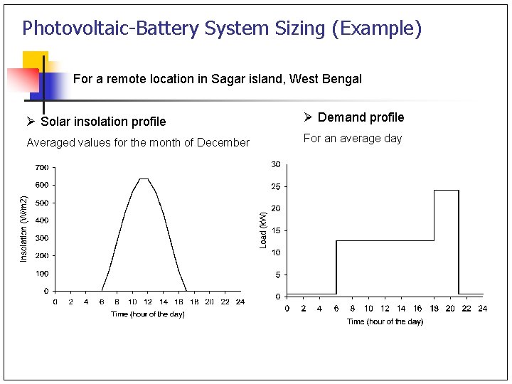
Photovoltaic-Battery System Sizing (Example) For a remote location in Sagar island, West Bengal Ø Solar insolation profile Ø Demand profile Averaged values for the month of December For an average day

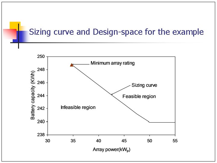
Sizing curve and Design-space for the example

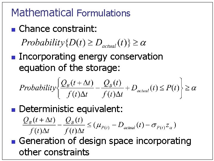
Mathematical Formulations n n Chance constraint: Incorporating energy conservation equation of the storage: Deterministic equivalent: Generation of design space incorporating other constraints

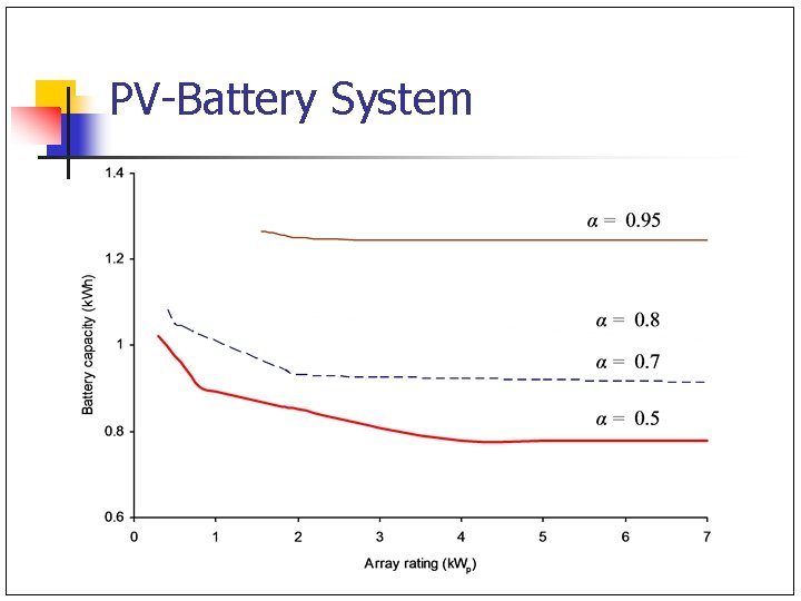
PV-Battery System

Solar Water Heaters Estimate potential for solar water heaters in a given area n Develop generic framework ‘Diffusion of Renewable Energy Technologies’ n

Factors Affecting Diffusion Of SWHS n n n n Location- Insolation Water Usage Pattern Cost of electricity Capital Cost Reliability Potential savings Subsidies/ Financial Incentives

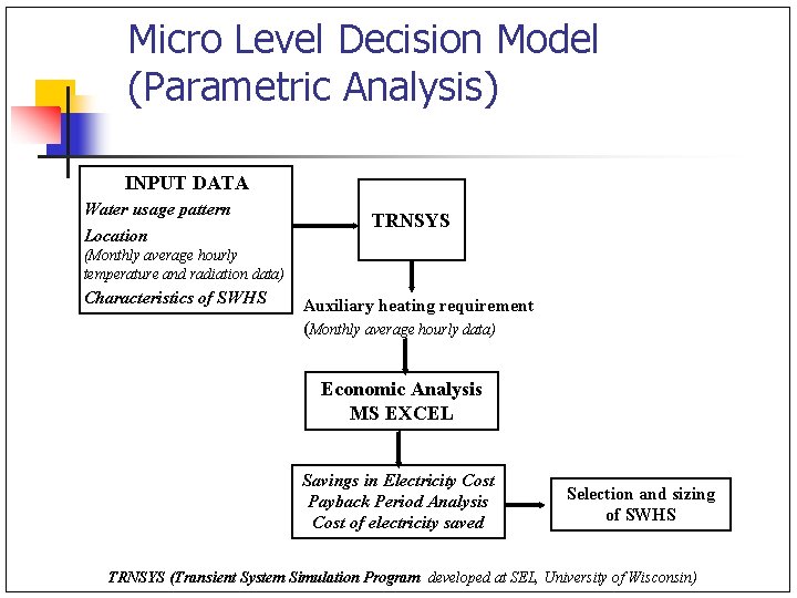
Micro Level Decision Model (Parametric Analysis) INPUT DATA Water usage pattern Location TRNSYS (Monthly average hourly temperature and radiation data) Characteristics of SWHS Auxiliary heating requirement (Monthly average hourly data) Economic Analysis MS EXCEL Savings in Electricity Cost Payback Period Analysis Cost of electricity saved Selection and sizing of SWHS TRNSYS (Transient System Simulation Program developed at SEL, University of Wisconsin)

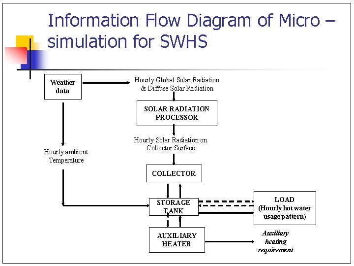
Information Flow Diagram of Micro – simulation for SWHS Weather data Hourly Global Solar Radiation & Diffuse Solar Radiation SOLAR RADIATION PROCESSOR Hourly ambient Temperature Hourly Solar Radiation on Collector Surface COLLECTOR STORAGE TANK LOAD (Hourly hot water usage pattern) AUXILIARY HEATER Auxiliary heating requirement

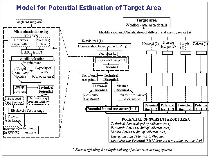
Model for Potential Estimation of Target Area Target area Weather data, area details Single end use point Micro simulation using TRNSYS Hot water Weather usage pattern data Identification and Classification of different end uses by sector ( i) Residential (1) Classification based on factors* (j) SIMULATION Auxiliary heating requirement Capacity of Target SWHS Auxiliary (Collector area) heating Technical Potential SWHS capacity Base load for heating Constraint: roof area availability Electricity/ fuel savings Price of electricity Investment for SWHS Economic viability Hospital (2) Nursing Homes (3) Hotels Others (5) (4) Sub-class (i, j) Single end use point Potential No. of end use points Technical Potential Economic Constraint Market Potential Constraint: market acceptance Potential for end use sector (i = 1) Potential for i = 2 for i = 3 Potential for i = 4 for i = 5 POTENTIAL OF SWHS IN TARGET AREA Technical Potential (m 2 of collector area) Economic Potential (m 2 of collector area) Market Potential (m 2 of collector area) Energy Savings Potential (k. Wh/year) Load Shaving Potential (k. Wh/ hour for a monthly average day) * Factors affecting the adoption/sizing of solar water heating systems

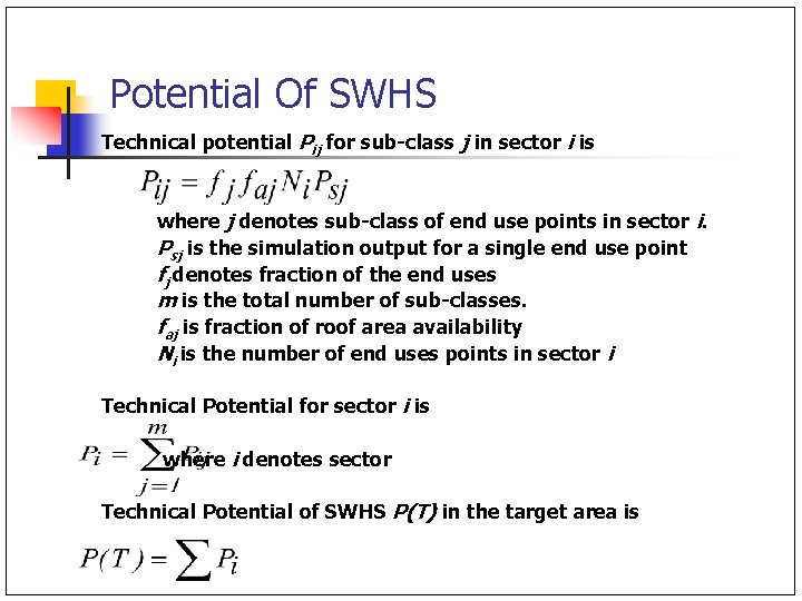
Potential Of SWHS Technical potential Pij for sub-class j in sector i is where j denotes sub-class of end use points in sector i. Psj is the simulation output for a single end use point fj denotes fraction of the end uses m is the total number of sub-classes. faj is fraction of roof area availability Ni is the number of end uses points in sector i Technical Potential for sector i is where i denotes sector Technical Potential of SWHS P(T) in the target area is

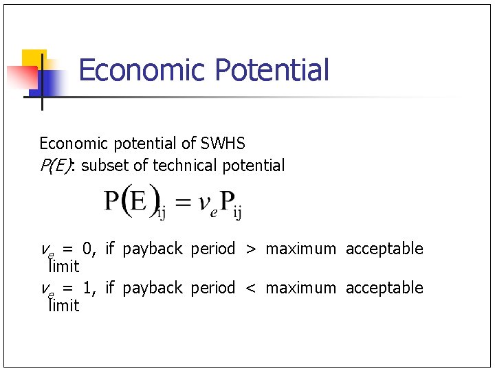
Economic Potential Economic potential of SWHS P(E): subset of technical potential ve = 0, if payback period > maximum acceptable limit ve = 1, if payback period < maximum acceptable limit

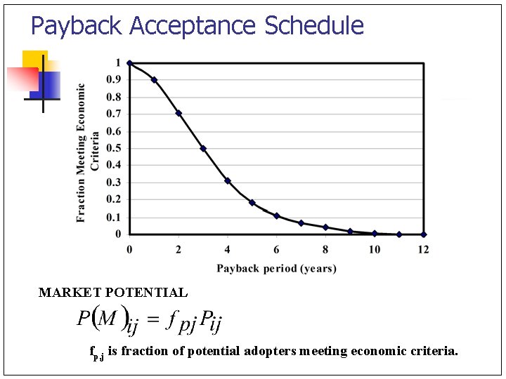
Payback Acceptance Schedule MARKET POTENTIAL fp, j is fraction of potential adopters meeting economic criteria.

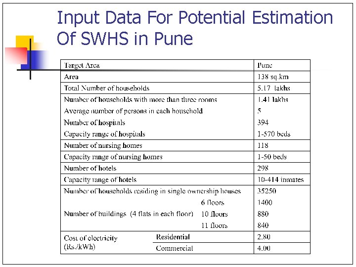
Input Data For Potential Estimation Of SWHS in Pune

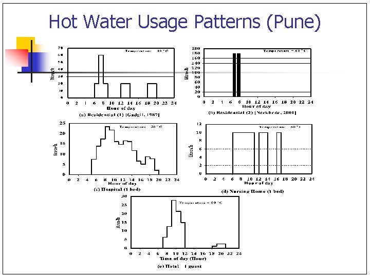
Hot Water Usage Patterns (Pune)

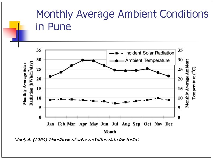
Monthly Average Ambient Conditions in Pune Mani, A. (1980) ‘Handbook of solar radiation data for India’.

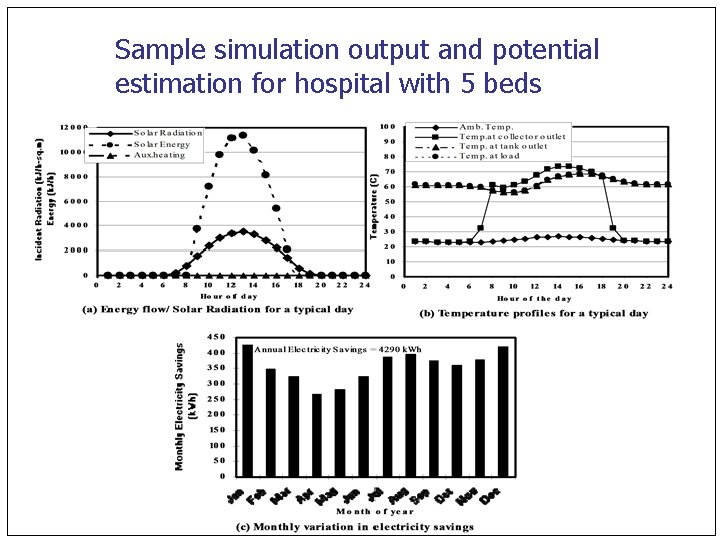
Sample simulation output and potential estimation for hospital with 5 beds

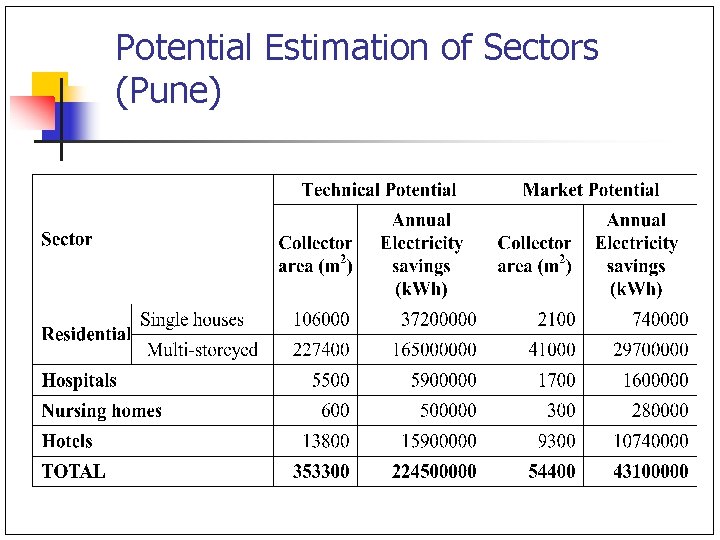
Potential Estimation of Sectors (Pune)

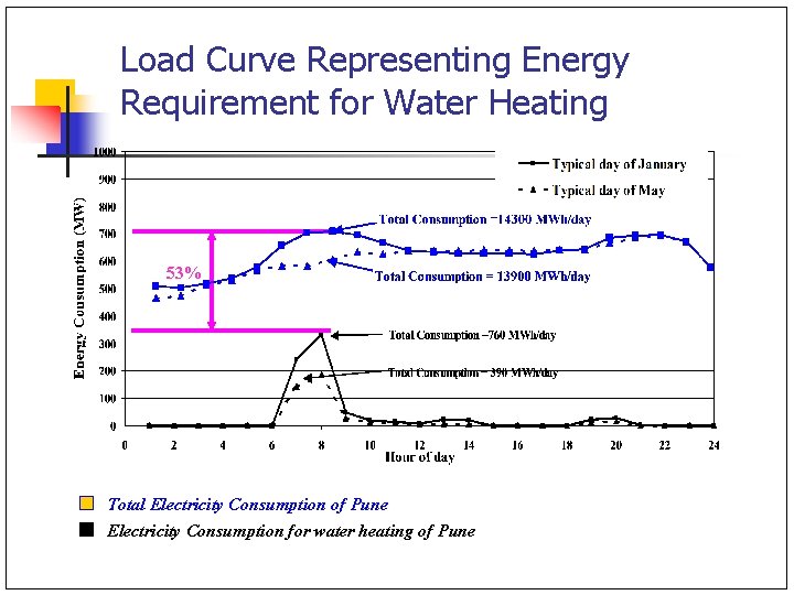
Load Curve Representing Energy Requirement for Water Heating 53% Total Electricity Consumption of Pune Electricity Consumption for water heating of Pune

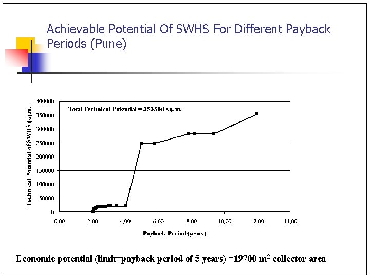
Achievable Potential Of SWHS For Different Payback Periods (Pune) Economic potential (limit=payback period of 5 years) =19700 m 2 collector area

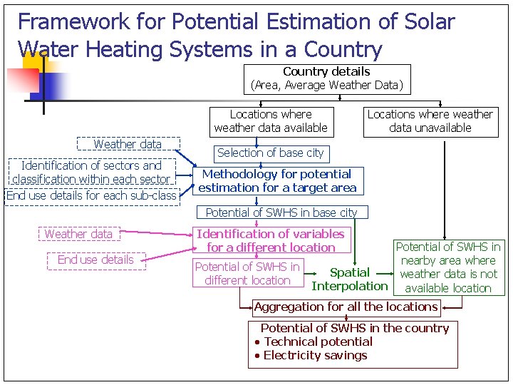
Framework for Potential Estimation of Solar Water Heating Systems in a Country details (Area, Average Weather Data) Locations where weather data available Weather data Identification of sectors and classification within each sector End use details for each sub-class Locations where weather data unavailable Selection of base city Methodology for potential estimation for a target area Potential of SWHS in base city Weather data End use details Identification of variables for a different location Potential of SWHS in nearby area where Spatial weather data is not Interpolation available location Aggregation for all the locations Potential of SWHS in the country · Technical potential · Electricity savings

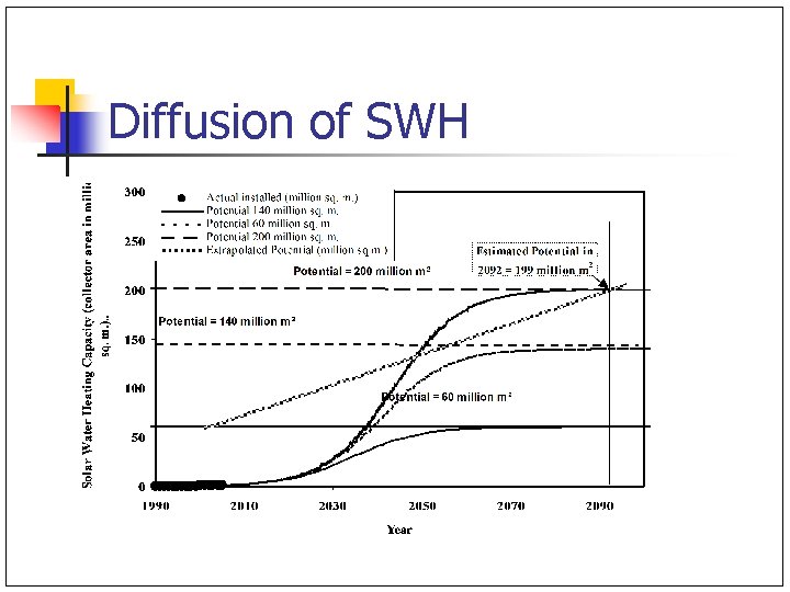
Diffusion of SWH

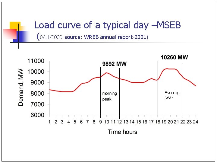
Load curve of a typical day –MSEB (8/11/2000 source: WREB annual report-2001) Evening peak

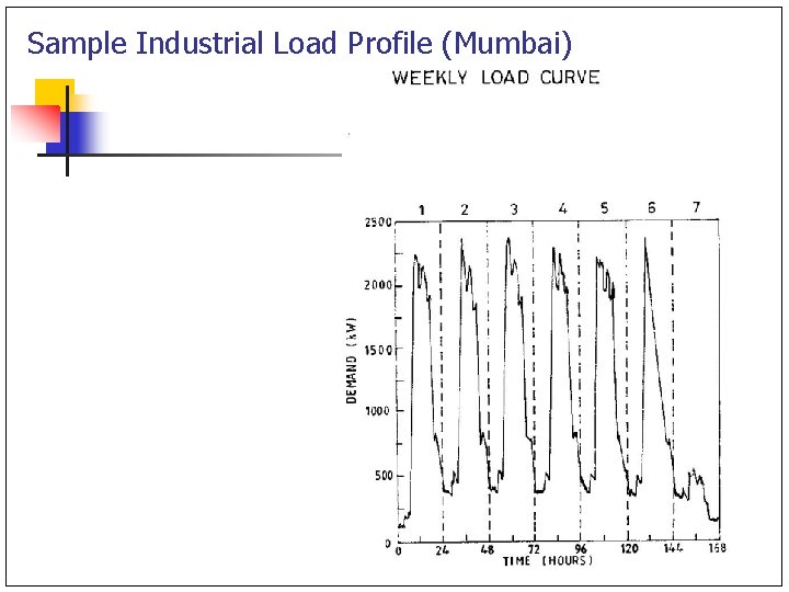
Sample Industrial Load Profile (Mumbai)

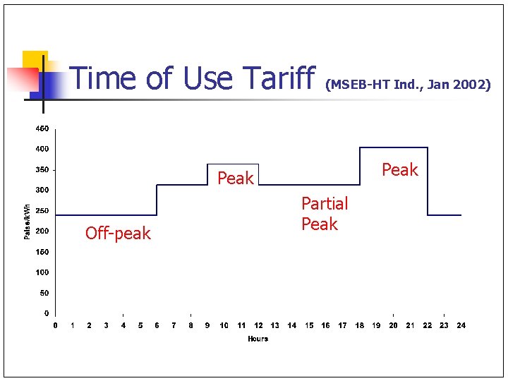
Time of Use Tariff (MSEB-HT Ind. , Jan 2002) Peak Off-peak Partial Peak

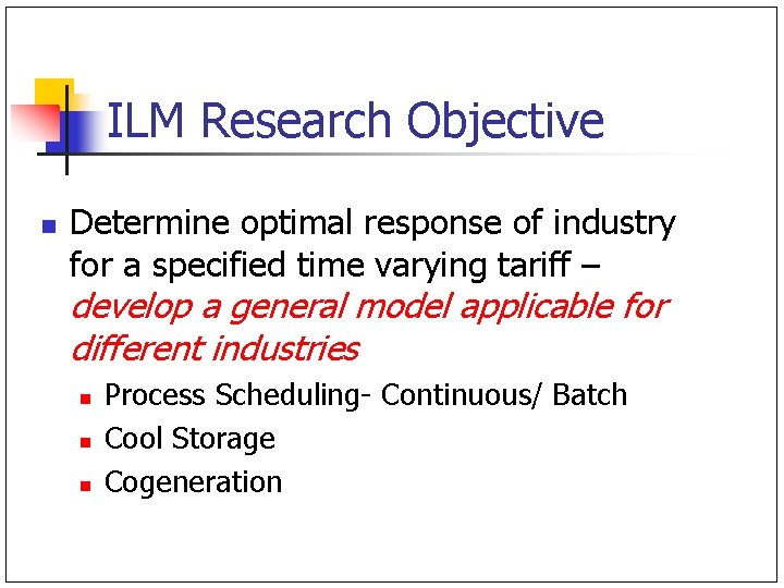
ILM Research Objective n Determine optimal response of industry for a specified time varying tariff – develop a general model applicable for different industries n n n Process Scheduling- Continuous/ Batch Cool Storage Cogeneration

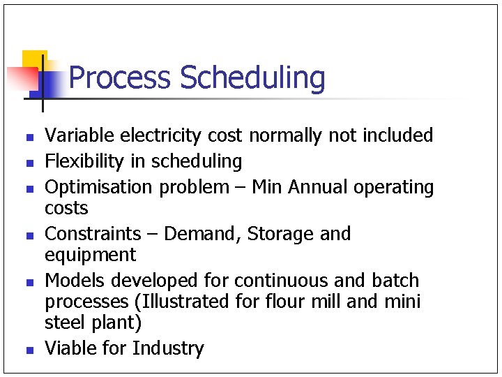
Process Scheduling n n n Variable electricity cost normally not included Flexibility in scheduling Optimisation problem – Min Annual operating costs Constraints – Demand, Storage and equipment Models developed for continuous and batch processes (Illustrated for flour mill and mini steel plant) Viable for Industry

Process Scheduling n n Batch processes- batch time, quantity, charging, discharging, power demand variation (load cycles) Raw material constraints, Allocation constraints, Storage constraints, Sequential Constraints, maintenance downtime

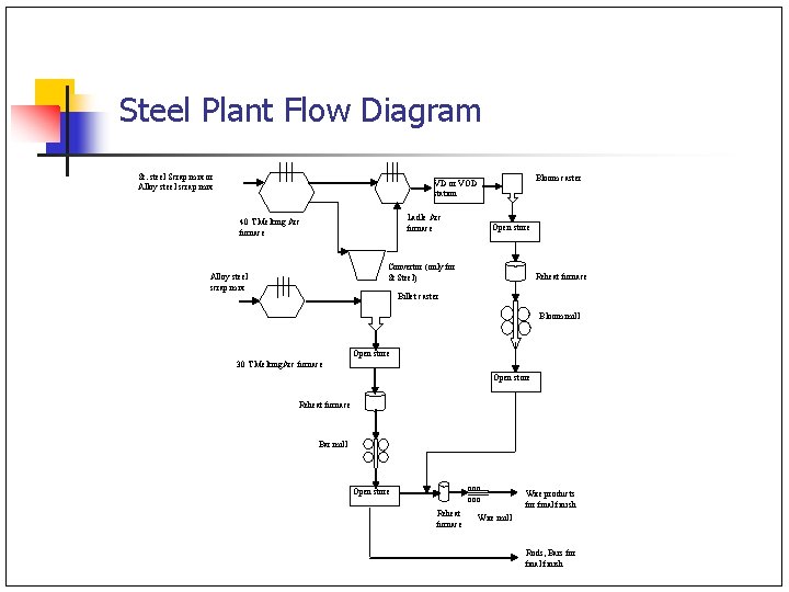
Steel Plant Flow Diagram St. steel Scrap mix or Alloy steel scrap mix Bloom caster VD or VOD station Ladle Arc furnace 40 T Melting Arc furnace Open store Convertor (only for St Steel) Alloy steel scrap mix Reheat furnace Billet caster Bloom mill Open store 30 T Melting. Arc furnace Open store Reheat furnace Bar mill ooo Open store Reheat furnace Wire products for final finish Wire mill Rods, Bars for final finish

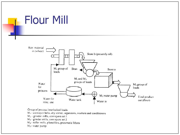
Flour Mill

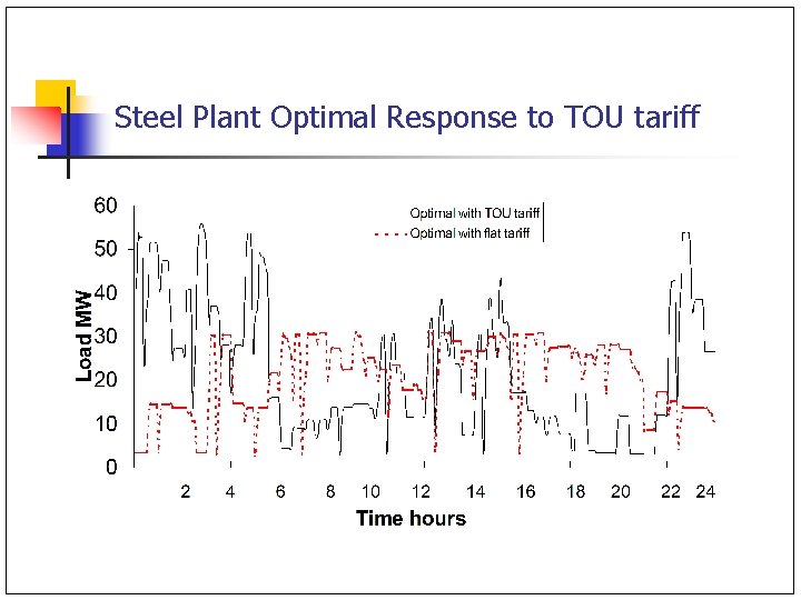
Steel Plant Optimal Response to TOU tariff

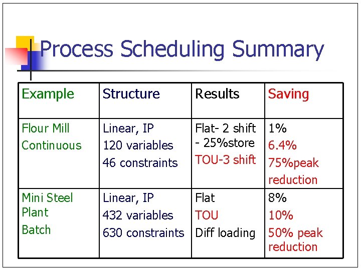
Process Scheduling Summary Example Structure Results Saving Flour Mill Continuous Linear, IP 120 variables 46 constraints Flat- 2 shift - 25%store TOU-3 shift 1% 6. 4% 75%peak reduction Mini Steel Plant Batch Linear, IP Flat 432 variables TOU 630 constraints Diff loading 8% 10% 50% peak reduction

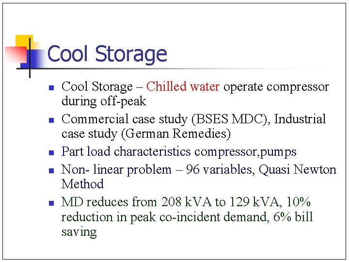
Cool Storage n n n Cool Storage – Chilled water operate compressor during off-peak Commercial case study (BSES MDC), Industrial case study (German Remedies) Part load characteristics compressor, pumps Non- linear problem – 96 variables, Quasi Newton Method MD reduces from 208 k. VA to 129 k. VA, 10% reduction in peak co-incident demand, 6% bill saving

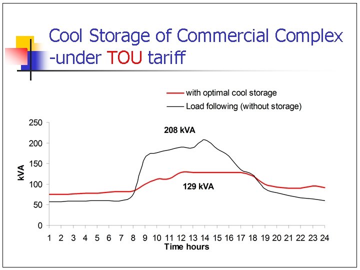
Cool Storage of Commercial Complex -under TOU tariff

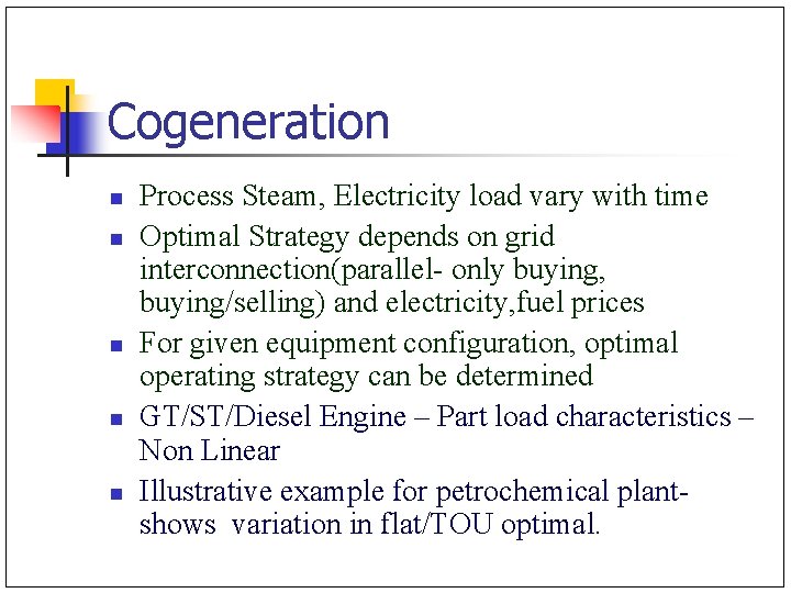
Cogeneration n n Process Steam, Electricity load vary with time Optimal Strategy depends on grid interconnection(parallel- only buying, buying/selling) and electricity, fuel prices For given equipment configuration, optimal operating strategy can be determined GT/ST/Diesel Engine – Part load characteristics – Non Linear Illustrative example for petrochemical plant- shows variation in flat/TOU optimal.

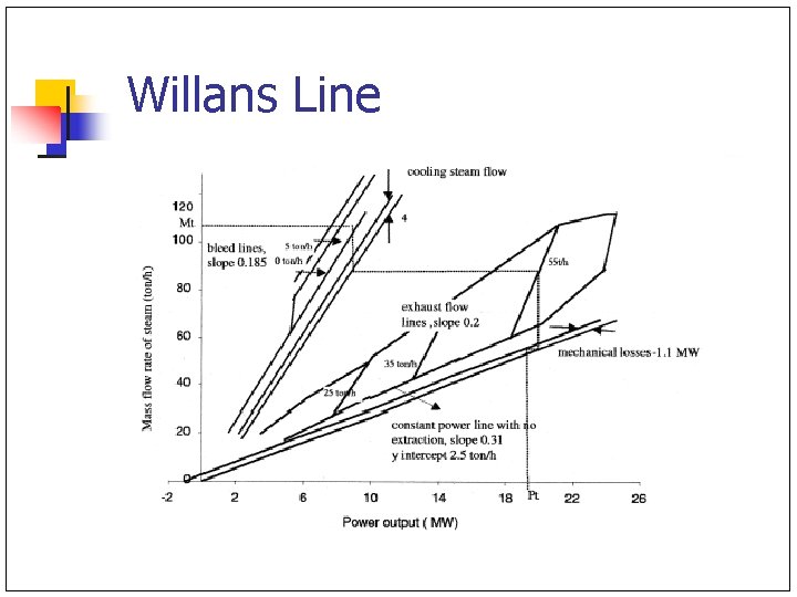
Willans Line

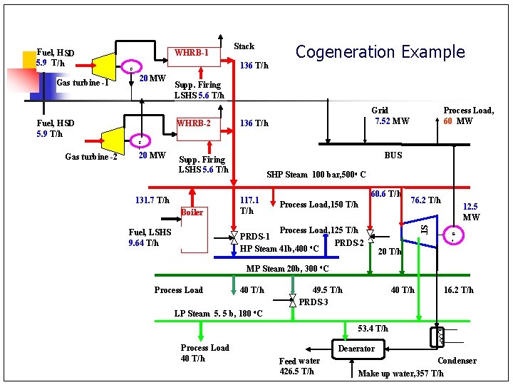
Fuel, HSD 5. 9 T/h Gas turbine -1 WHRB-1 136 T/h G 1 Stack 20 MW Fuel, HSD 5. 9 T/h Cogeneration Example Supp. Firing LSHS 5. 6 T/h WHRB-2 Grid 7. 52 MW 136 T/h Process Load, 60 MW G Gas turbine -2 1 20 MW BUS Supp. Firing LSHS 5. 6 T/h 131. 7 T/h Boiler SHP Steam 100 bar, 500 o C 117. 1 T/h 60. 6 T/h Process Load, 150 T/h ST Process Load, 125 T/h PRDS-1 PRDS-2 HP Steam 41 b, 400 o. C Fuel, LSHS 9. 64 T/h 76. 2 T/h 12. 5 MW G 4 20 T/h MP Steam 20 b, 300 o. C Process Load 40 T/h 49. 5 T/h PRDS-3 40 T/h 16. 2 T/h LP Steam 5. 5 b, 180 o. C 53. 4 T/h Process Load 40 T/h Deaerator Feed water 426. 5 T/h Condenser Make up water, 357 T/h

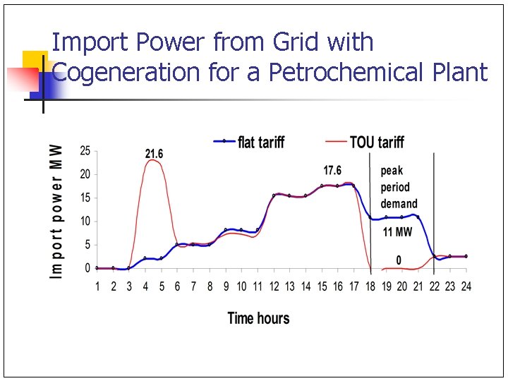
Import Power from Grid with Cogeneration for a Petrochemical Plant

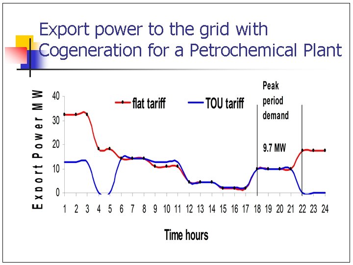
Export power to the grid with Cogeneration for a Petrochemical Plant

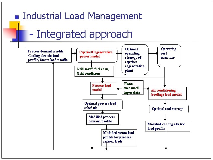
n Industrial Load Management - Integrated approach Process demand profile, Cooling electric load profile, Steam load profile Captive/Cogeneration power model Grid tariff, fuel costs, Grid conditions Process load model Optimal operating strategy of captive/ cogeneration plant Plant/ measured input data Optimal process load schedule Modified process demand profile Modified steam load profile for process related loads Operating cost structure Air conditioning (cooling) load model Optimal cool storage Modified cooling electric load profile

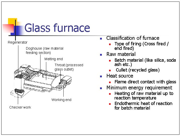
Glass furnace n Regenerator Classification of furnace n Doghouse (raw material feeding section) n Melting end Raw material n Throat (processed glass outlet) n n Flame direct contact with glass Minimum energy requirement n Working end Checker work Batch material (like silica, soda ash etc. ) Cullet (recycled glass) Heat source n n Type of firing (Cross fired / end fired) n Heating of raw material up to reaction temperature Endothermic heat of reaction for batch material

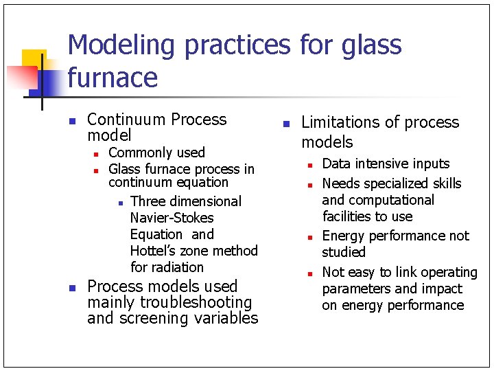
Modeling practices for glass furnace n Continuum Process model n n n Commonly used Glass furnace process in continuum equation n Three dimensional Navier-Stokes Equation and Hottel’s zone method for radiation Process models used mainly troubleshooting and screening variables n Limitations of process models n n Data intensive inputs Needs specialized skills and computational facilities to use Energy performance not studied Not easy to link operating parameters and impact on energy performance

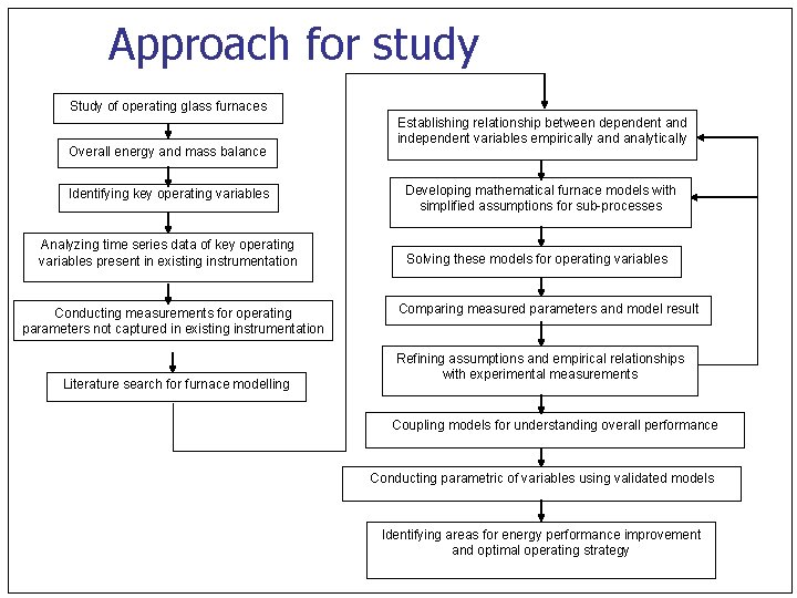
Approach for study Study of operating glass furnaces Overall energy and mass balance Identifying key operating variables Analyzing time series data of key operating variables present in existing instrumentation Conducting measurements for operating parameters not captured in existing instrumentation Literature search for furnace modelling Establishing relationship between dependent and independent variables empirically and analytically Developing mathematical furnace models with simplified assumptions for sub-processes Solving these models for operating variables Comparing measured parameters and model result Refining assumptions and empirical relationships with experimental measurements Coupling models for understanding overall performance Conducting parametric of variables using validated models Identifying areas for energy performance improvement and optimal operating strategy

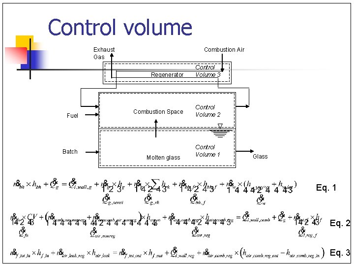
Control volume Exhaust Gas Fuel Batch Combustion Air Regenerator Control Volume 3 Combustion Space Control Volume 2 Molten glass Control Volume 1 Glass Eq. 1 Eq. 2 Eq. 3

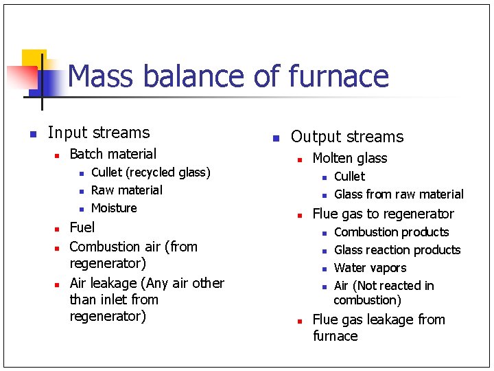
Mass balance of furnace n Input streams n Batch material n n n Cullet (recycled glass) Raw material Moisture Fuel Combustion air (from regenerator) Air leakage (Any air other than inlet from regenerator) n Output streams n Molten glass n n n Flue gas to regenerator n n n Cullet Glass from raw material Combustion products Glass reaction products Water vapors Air (Not reacted in combustion) Flue gas leakage from furnace

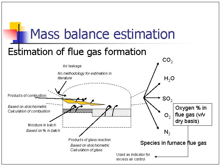
Mass balance estimation Estimation of flue gas formation CO 2 Air leakage No methodology for estimation in literature H 2 O Products of combustion SO 2 Based on stoichiometric Calculation of combustion O 2 Moisture in batch Based on % in batch Oxygen % in flue gas (v/v dry basis) N 2 Products of glass reaction Based on stoichiometric Calculation of glass Species in furnace flue gas Used as indicator for excess air control

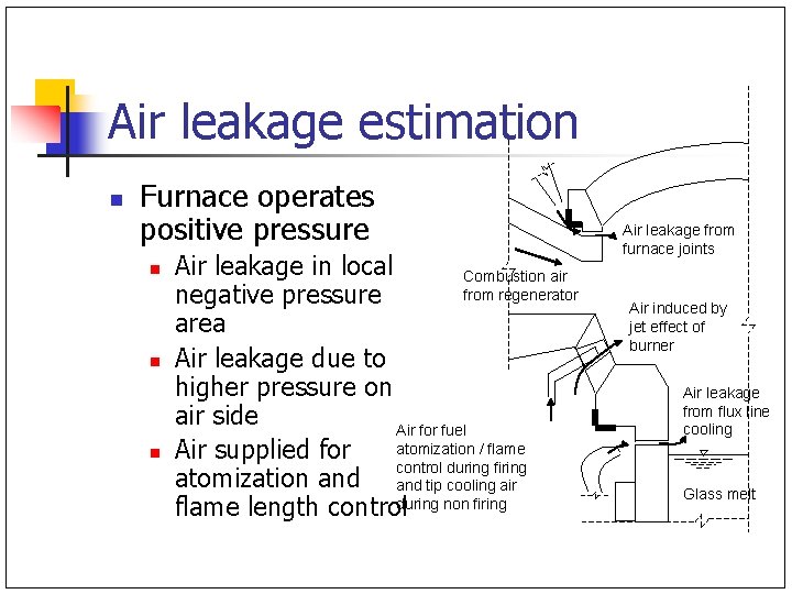
Air leakage estimation n Furnace operates positive pressure n n n Air leakage in local Combustion air from regenerator negative pressure area Air leakage due to higher pressure on air side Air for fuel atomization / flame Air supplied for control during firing atomization and tip cooling air flame length controlduring non firing Air leakage from furnace joints Air induced by jet effect of burner Air leakage from flux line cooling Glass melt

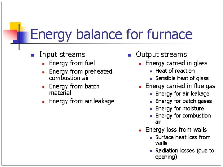
Energy balance for furnace n Input streams n n Energy from fuel Energy from preheated combustion air Energy from batch material Energy from air leakage n Output streams n Energy carried in glass n n n Energy carried in flue gas n n n Heat of reaction Sensible heat of glass Energy air for for air leakage batch gases moisture combustion Energy loss from walls n n Surface heat loss from walls Radiation losses (due to opening)

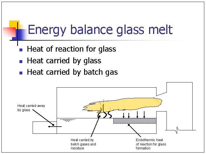
Energy balance glass melt n n n Heat of reaction for glass Heat carried by batch gas Heat carried away by glass Heat carried by batch gases and moisture Endothermic heat of reaction for glass formation

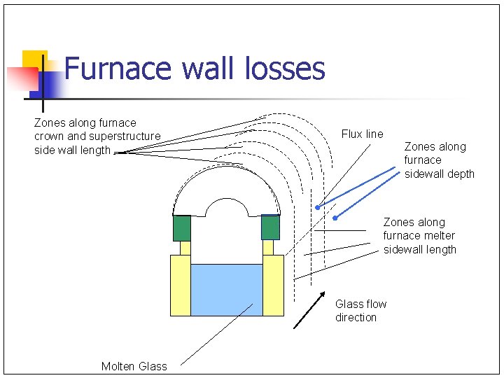
Furnace wall losses Zones along furnace crown and superstructure side wall length Flux line Zones along furnace sidewall depth Zones along furnace melter sidewall length Glass flow direction Molten Glass

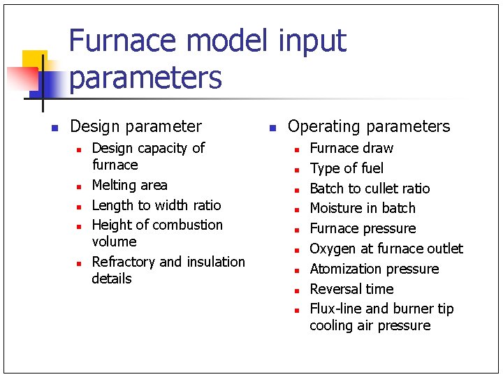
Furnace model input parameters n Design parameter n n n Design capacity of furnace Melting area Length to width ratio Height of combustion volume Refractory and insulation details n Operating parameters n n n n n Furnace draw Type of fuel Batch to cullet ratio Moisture in batch Furnace pressure Oxygen at furnace outlet Atomization pressure Reversal time Flux-line and burner tip cooling air pressure

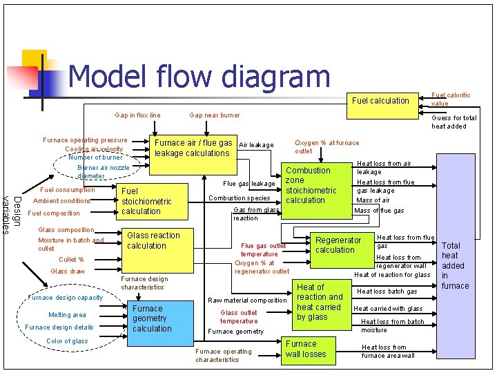
Model flow diagram Fuel calculation Gap in flux line Furnace operating pressure Cooling air velocity Number of burner Burner air nozzle diameter Fuel consumption Design variables Ambient conditions Fuel composition Glass composition Moisture in batch and cullet Fuel stoichiometric calculation Glass reaction calculation Furnace design details Flue gas leakage Combustion species Oxygen % at furnace outlet Combustion zone stoichiometric calculation Gas from glass reaction Flue gas outlet temperature Oxygen % at regenerator outlet Furnace design characteristics Furnace design capacity Melting area Guess for total heat added Furnace air / flue gas Air leakage calculations Cullet % Glass draw Gap near burner Raw material composition Furnace geometry calculation Glass outlet temperature Furnace operating characteristics Heat loss from air leakage Heat loss from flue gas leakage Mass of air Mass of flue gas Regenerator calculation Heat loss from flue gas Heat loss from regenerator wall Heat of reaction for glass Heat of reaction and heat carried by glass Furnace geometry Color of glass Fuel calorific value Furnace wall losses Heat loss batch gas Heat carried with glass Heat loss from batch moisture Heat loss from furnace area wall Total heat added in furnace

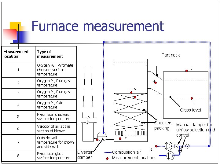
Furnace measurement Measurement location Type of measurement 1 Oxygen % , Pyrometer checkers surface temperature 2 Oxygen %, Flue gas temperature 3 Oxygen %, Flue gas temperature 4 Oxygen %, Skin temperature 5 Pyrometer checkers surface temperature 6 Velocity of air at the suction of blower 7 Outside wall temperature for crown and side wall 8 Pyrometer glass surface temperature Port neck 7 4 5 1 8 Glass level Checkers Manual damper for packing airflow selection and control 2 3 Diverter damper 6 Combustion air Measurement locations

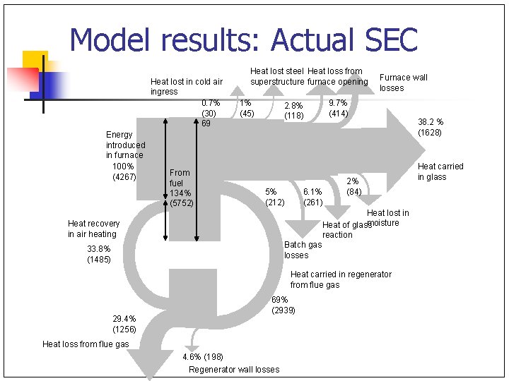
Model results: Actual SEC Heat lost in cold air ingress 0. 7% (30) 69 Energy introduced in furnace 100% (4267) From fuel 134% (5752) Heat lost steel Heat loss from superstructure furnace opening 1% (45) 2. 8% (118) 5% (212) 6. 1% (261) Furnace wall losses 9. 7% (414) 2% (84) Heat lost in moisture Heat of glass reaction Batch gas losses Heat recovery in air heating 33. 8% (1485) Heat carried in regenerator from flue gas 29. 4% (1256) 69% (2939) Heat loss from flue gas 4. 6% (198) Regenerator wall losses 38. 2 % (1628) Heat carried in glass

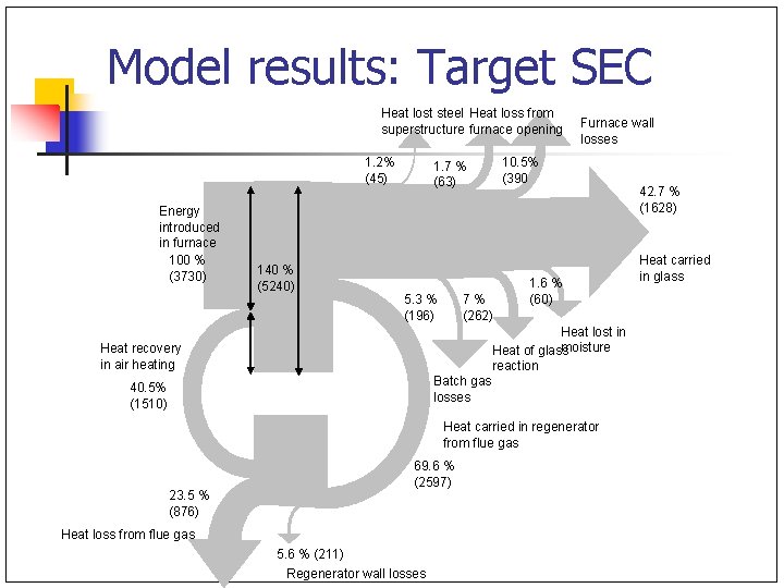
Model results: Target SEC Heat lost steel Heat loss from superstructure furnace opening 1. 2% (45) Energy introduced in furnace 100 % (3730) 140 % (5240) 1. 7 % (63) 5. 3 % (196) 7 % (262) Furnace wall losses 10. 5% (390 1. 6 % (60) Heat lost in moisture Heat of glass reaction Batch gas losses Heat recovery in air heating 40. 5% (1510) Heat carried in regenerator from flue gas 23. 5 % (876) 69. 6 % (2597) Heat loss from flue gas 5. 6 % (211) Regenerator wall losses 42. 7 % (1628) Heat carried in glass

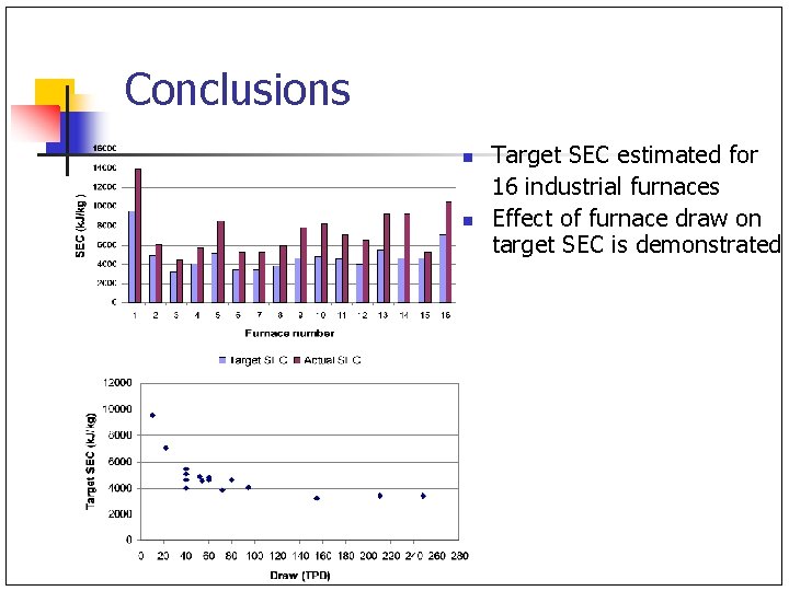
Conclusions n n Target SEC estimated for 16 industrial furnaces Effect of furnace draw on target SEC is demonstrated

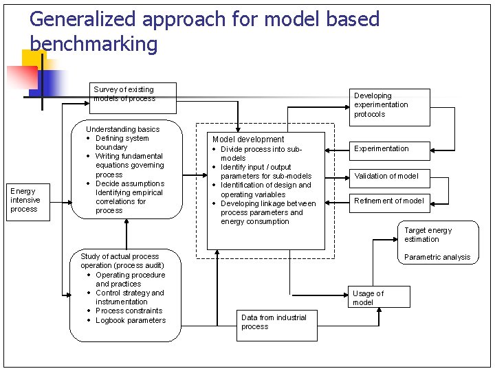
Generalized approach for model based benchmarking Survey of existing models of process Energy intensive process Understanding basics · Defining system boundary · Writing fundamental equations governing process · Decide assumptions Identifying empirical correlations for process Developing experimentation protocols Model development · Divide process into submodels · Identify input / output parameters for sub-models · Identification of design and operating variables · Developing linkage between process parameters and energy consumption Experimentation Validation of model Refinement of model Target energy estimation Study of actual process operation (process audit) · Operating procedure and practices · Control strategy and instrumentation · Process constraints · Logbook parameters Parametric analysis Usage of model Data from industrial process

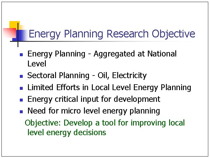
Energy Planning Research Objective Energy Planning - Aggregated at National Level n Sectoral Planning - Oil, Electricity n Limited Efforts in Local Level Energy Planning n Energy critical input for development n Need for micro level energy planning Objective: Develop a tool for improving local level energy decisions n

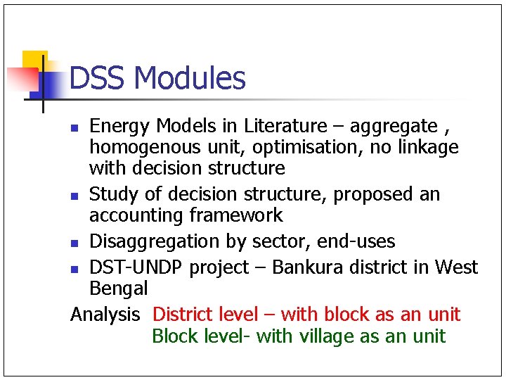
DSS Modules Energy Models in Literature – aggregate , homogenous unit, optimisation, no linkage with decision structure n Study of decision structure, proposed an accounting framework n Disaggregation by sector, end-uses n DST-UNDP project – Bankura district in West Bengal Analysis District level – with block as an unit Block level- with village as an unit n

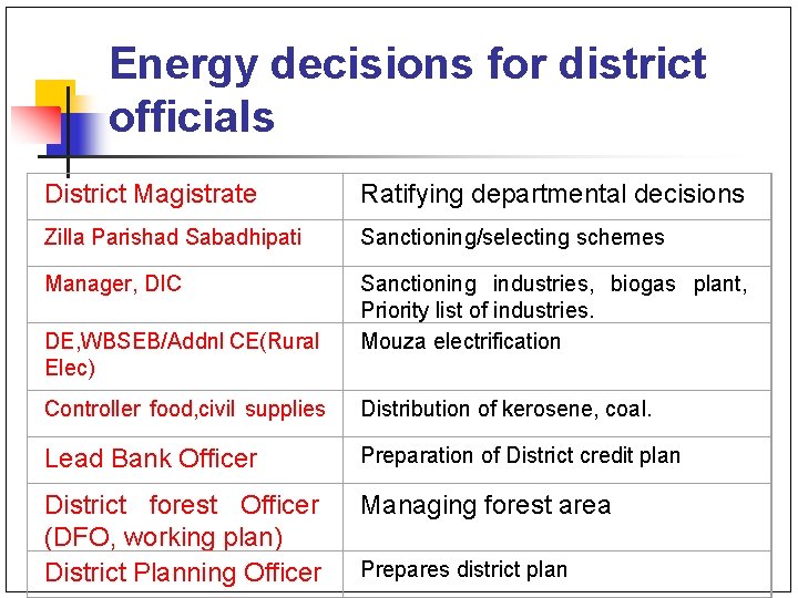
Energy decisions for district officials District Magistrate Ratifying departmental decisions Zilla Parishad Sabadhipati Sanctioning/selecting schemes Manager, DIC Sanctioning industries, biogas plant, Priority list of industries. Mouza electrification DE, WBSEB/Addnl CE(Rural Elec) Controller food, civil supplies Distribution of kerosene, coal. Lead Bank Officer Preparation of District credit plan District forest Officer (DFO, working plan) District Planning Officer Managing forest area Prepares district plan

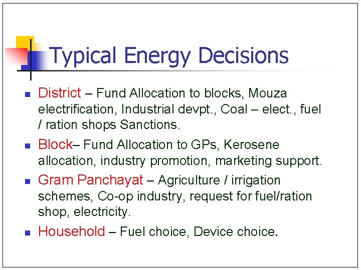
Typical Energy Decisions n District – Fund Allocation to blocks, Mouza electrification, Industrial devpt. , Coal – elect. , fuel / ration shops Sanctions. n Block– Fund Allocation to GPs, Kerosene allocation, industry promotion, marketing support. n Gram Panchayat – Agriculture / irrigation schemes, Co-op industry, request for fuel/ration shop, electricity. n Household – Fuel choice, Device choice.

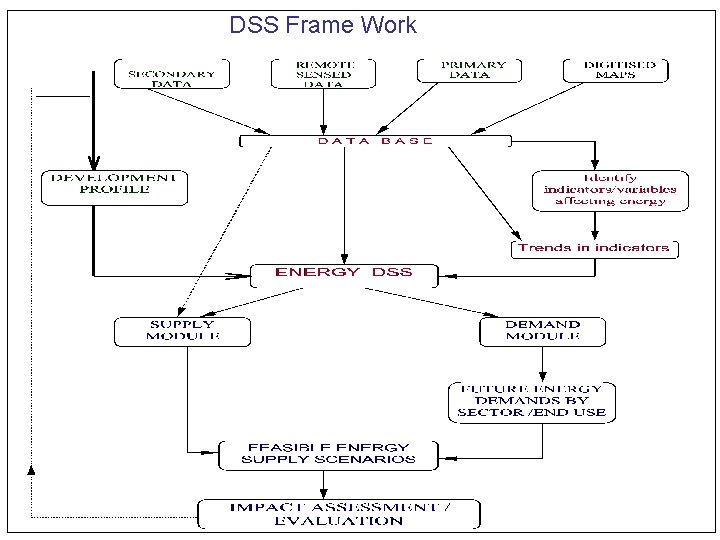
DSS Frame Work

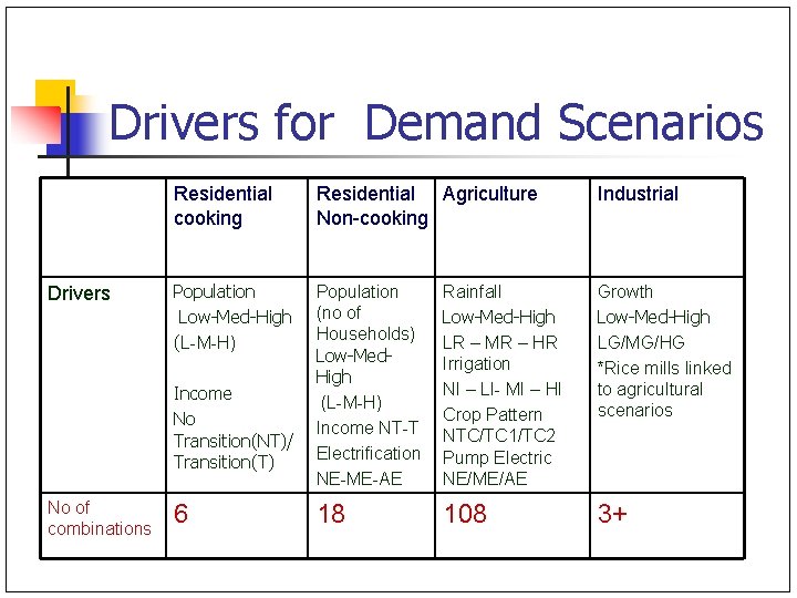
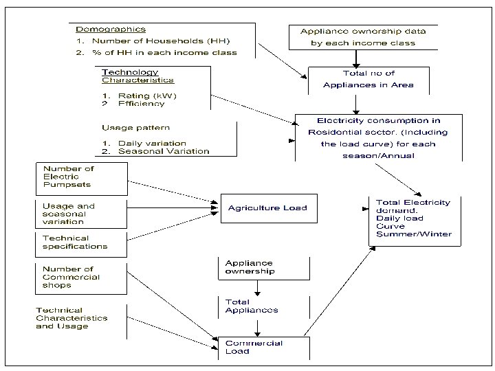
Drivers for Demand Scenarios Drivers Residential cooking Residential Agriculture Non-cooking Industrial Population Low-Med-High (L-M-H) Population (no of Households) Low-Med. High (L-M-H) Income NT-T Electrification NE-ME-AE Rainfall Low-Med-High LR – MR – HR Irrigation NI – LI- MI – HI Crop Pattern NTC/TC 1/TC 2 Pump Electric NE/ME/AE Growth Low-Med-High LG/MG/HG *Rice mills linked to agricultural scenarios 18 108 3+ Income No Transition(NT)/ Transition(T) No of combinations 6

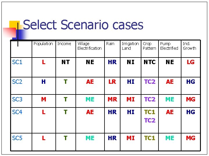
Select Scenario cases Population Income Village Electrification SC 1 L NT NE SC 2 H T SC 3 M SC 4 SC 5 Rain Irrigation Land Crop Pattern Pump Electrified Ind. Growth HR NI NTC NE LG AE LR HI TC 2 AE HG T ME MR MI TC 2 ME MG L T AE HR HI TC 1 TC 2 AE HG L T ME HR MI TC 1 ME MG

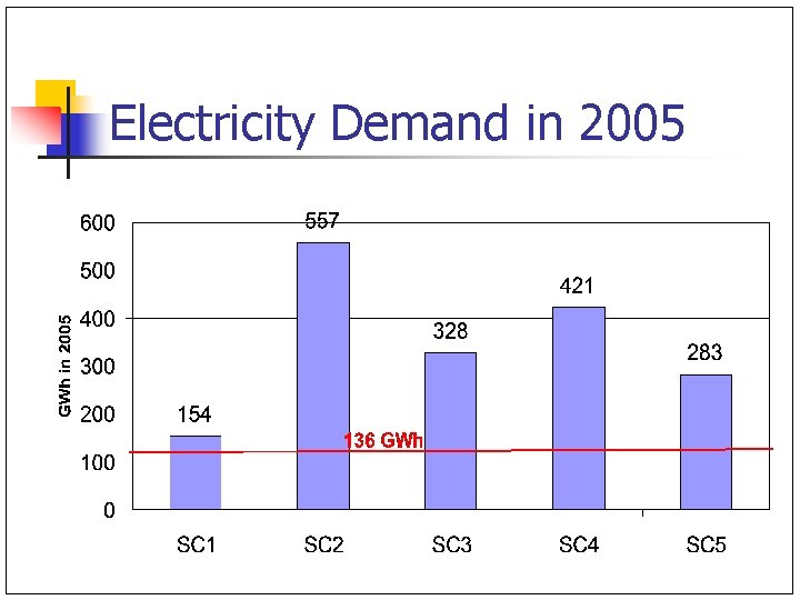
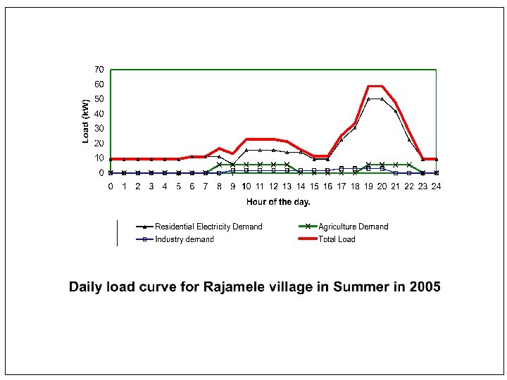
Electricity Demand in 2005

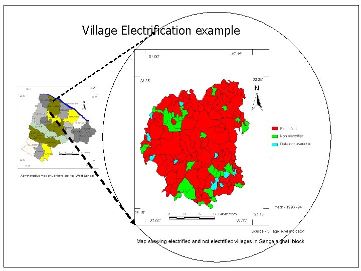
Village Electrification example

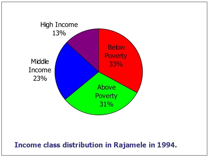
Income class distribution in Rajamele in 1994.

DSS Capability/Use n n n Energy Quantification- from data already available/collected by Govt Assess impacts of development paths Quantify future commercial fuel demands – elec/coal/LPG/kerosene Rural Electrification- Load Profile Estimation, Sizing, Option Selection, Impact Assessment Spatial Representation of results Classification of areas as biomass surplus/deficit

Summing Up n n n Examples – illustrate variety of optimisation/ simulation models for energy sector Decision context and model formulation critical Reality check - Applicability Generalisation important but. . Data intensity and uncertainty

Acknowledgment Indu Pillai S. Ashok Ph. D - 2003 Ph. D - 2008 Vishal S. Ph. D. - 2008 Sandeep Phulluke, Sagar Kasar, Abhijit Bhure, Amit Khare, Jagdish DSS Project Staff (2004 -2006) U. N. Gaitonde Faculty Balkrishna Surve Project Assistant Arun P. Ph. D. - 2009 Mel George A. M. Tech - Ongoing Santanu B. Faculty Manojkumar M. V. M. Tech - Ongoing Thank you

References n n n Ashok. S and R. Banerjee , “An Optimisation model for Industrial Load management”, IEEE Trans on Power Systems, Vol. 16, No. 4, Nov. 2001, pp 879 -884. Ashok S and R. Banerjee , Optimal Operation of Industrial Cogeneration for Load Management, IEEE Trans on Power Systems, Vol. 18, No. 2, MAY 2003. Ashok. S and R. Banerjee, Optimal cool storage capacity for load management , Energy, Vol. 28, pp 115 -126, 2003. Vishal S, U. N. Gaitonde, R Banerjee. , “Model based energy benchmarking for glass furnace”, Energy Conversion and Management, Vol. 48, pp 2718 -2738, 2007. R. Banerjee, A. B. Inamdar, S. Phulluke, B. Pateriya, “Decision Support System for Energy Planning in a District”, Economic and Political Weekly, Vol. 34, No. 50, pp 3545 -3552, 1999. R. Banerjee, Rahul Pandey, Abhijit Bhure and Sandeep Phulluke , “Electricity Demand Estimation for Village Electrification ”, Proceedings of National Renewable Energy Conference , IIT Bombay, Nov. 30 -Dec. 2 , 2000. Rahul Pandey, R. Banerjee, Abhijit Bhure and Sandeep Phulluke , “Framework for Design and Evaluation of Electric Supply Options for a rural area”, Proceedings of National Renewable Energy Conference , IIT Bombay, Nov. 30 -Dec. 2 , 2000. Arun P. , Santanu Bandyopadhyay and R. Banerjee, ‘Sizing curve for design of isolated power systems’, Energy for Sustainable Development, Volume XI, No. 4, December 2007. Indu R. Pillai and R. Banerjee, ‘Methodology for estimation of potential for solar water heating in a target area’, Solar Energy, Vol. 8, No. 2, pp 162 -17, 2007. George, R. Banerjee, Analysis of impacts of wind integration in the Tamil Nadu grid, in press, Energy Policy UK Wind speed data: GWEFR Cyf Hourly-mean wind speed datasets for sites in the European Wind Atlas, available at http: //www. gwefr. co. uk/datasets. htm UK load curves: Demand Data, UK National Grid, available at http: //www. nationalgrid. com/uk/Electricity/Data/