Modelling Magnetic Reconnection and Nanoflare Heating in the

Modelling Magnetic Reconnection and Nanoflare Heating in the Solar Corona The Coronal Heating Problem George Biggs Advisors: Mahboubeh Asgari-Targhi & Nicole Schanche

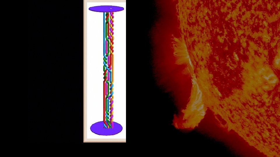
Why is the corona so hot? Two main complementary theories: Alfvenic turbulence (1 -3 MK, stable heating) Flare heating (3 -10 MK, rapid dynamic heating) Nanoflare heating can be influenced by Alfvenic turbulence Image: National Geographic 2011/06. EUV view.

Why Nanoflares? • Hudson (1990) explored microflares • Follow a power law with parameter of -1. 8, this is too low to explain the observed heating • Concluded a power law fit of over -2 is required

Magnetic Reconnection • Removes one crossing • Depends on critical crossing number • Only occurs in highly stressed situations

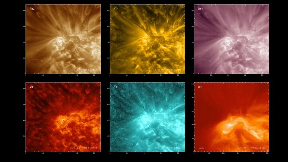
Magnetic Energy and Crossing Number Efree ∝ B min = 381. 05 Gauss Radius = 191. 7 km Length = 43. 8 Mm Image created using non-linear force free field fitting in CMS, HI-C data, 193 Å

Braidwords -Modelling braided fluxtubes • Complex crossings can be represented by a ‘braidword’ • Braidword corresponds to string of integers representing crossings Image on right (1, 3, 1, -4, 2, -4, 3, -2, -4) Images: Braidword examples from mathworld. wolfram. com

Avalanche Model • Analogy is a sand pile, once criticality is reached a small addition triggers avalanche • Can be applied to reconnection • In reconnection twisting motions of foot points are “grains of sand” being added

Reconnection In Action • Initial braidword {-1, -3, -1, 4, -2, 4, 4, -3, 2, 4, 4, -2, 1, 1, 1, -3, -2, 3, -1, -1, 2, -4, -4, -2, 3, -4, -4, 2, -4} • First reconnection occurs removing -2 crossing • Final braidword {-1, -3, -1}

Methods and Predictions • Expect a power law distribution • Initial parameters (B min, length, diameter) from the previously shown non-linear force free field modelling gives minimum crossing number • Found parameters for energy simulation by running reconnection simulation with parameters optimised through repeated trials

Finding Parameters • Analysed the results to see what the best fit was • Braidsize 10000, Reconnections 10000, Runs 500, Power Law -3. 41401 • Braidsize 500, Reconnections 1000, runs 500, Power Law = -3. 02347

Results Found power law fit as expected, approx. -2. 8

How This Dynamic Approach Differs • Zirken&Cleveland(1992) modelled nanoflares using grid randomly depositing energy • Longcope&Noonen(2000) also uses grid but evenly spaces opposite poles • Both have shortcomings avoided in this analysis

Comparison to Observation • Analysed the Hi-C (High-Resolution Coronal Imager)region to determine the number of flares in the two day period surrounding Hi-C • Expect distribution in types of flares with smaller more likely consistent with power law

Results Of Observations Distribution of Flare Intensities 25 20 Strength Of Event 15 10 5 0 7/9/12 15: 36 7/10/12 3: 36 7/10/12 15: 36 7/11/12 3: 36 7/11/12 15: 36 Time Of Event 7/12/12 3: 36 7/12/12 15: 36 7/13/12 3: 36

Past and Future • Updated modelling of reconnection to include avalanche model • Ran simulations using this updated model and found a power law as expected • To the future: Increase sophistication of model further by including internal twist

Acknowledgments Advisors Dr Mahboubeh Asgari-Targhi & Nicole Schanche and help from Patrick Mc. Cauley Dr. Henry “Trae” Winter, Dr. Kathy Reeves and the REU programme. NSF-REU solar physics programme at SAO, grant number AGS-1263241. AIA contract SP 02 H 1701 R from Lockheed-Martin to SAO. We acknowledge the High resolution Coronal Imager instrument team for making the flight data publicly available. MSFC/NASA led the mission and partners include the Smithsonian Astrophysical Observatory in Cambridge, Mass. ; Lockheed Martin's Solar Astrophysical Laboratory in Palo Alto, Calif. ; the University of Central Lancashire in Lancashire, England; and the Lebedev Physical Institute of the Russian Academy of Sciences in Moscow.