Modelled and measured stand transpiration and canopy conductance

Modelled and measured stand transpiration and canopy conductance of an Australian native forest Rhys Whitley 1, 2, 3, Melanie Zeppel 1, 2, Belinda Medlyn 4, Derek Eamus 1, 2 1 Institute for Water and Environmental Resource Management, University of Technology Sydney 2 Department of Environmental Sciences, University of Technology Sydney 3 Department of Physics and Advanced Materials, University of Technology Sydney 4 Department of Biological Sciences, Macquarie University UTS University of Technology, Sydney Institute for Water and Environmental Resource Management

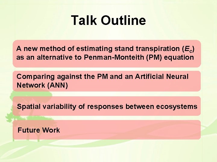
Talk Outline A new method of estimating stand transpiration (Ec) as an alternative to Penman-Monteith (PM) equation Comparing against the PM and an Artificial Neural Network (ANN) Spatial variability of responses between ecosystems Future Work

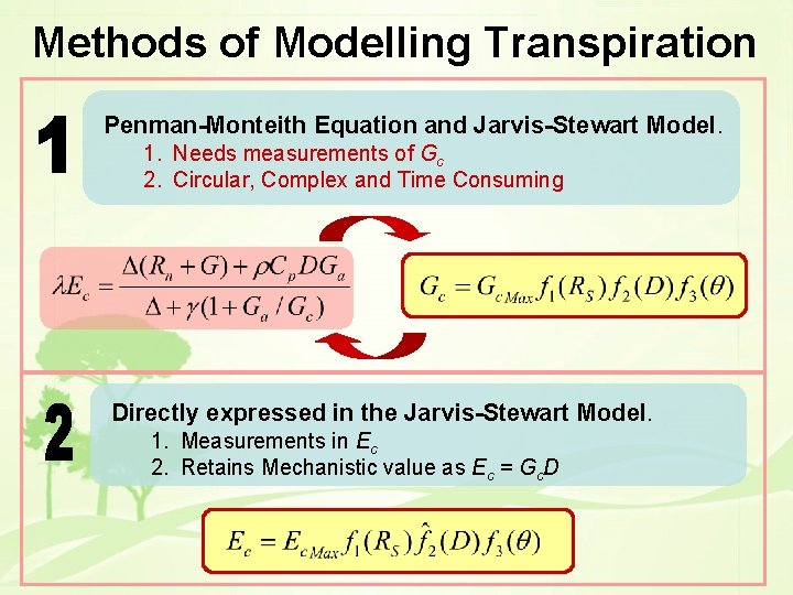
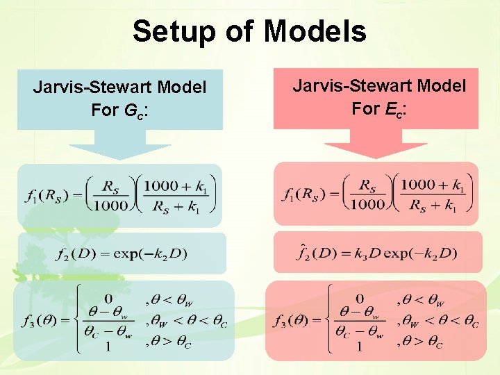
Methods of Modelling Transpiration Penman-Monteith Equation and Jarvis-Stewart Model. 1. Needs measurements of Gc 2. Circular, Complex and Time Consuming Directly expressed in the Jarvis-Stewart Model. 1. Measurements in Ec 2. Retains Mechanistic value as Ec = Gc. D

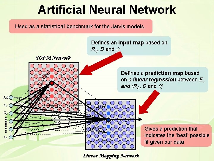
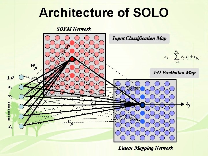
Artificial Neural Network Used as a statistical benchmark for the Jarvis models. Defines an input map based on RS, D and q SOFM Network Defines a prediction map based on a linear regression between Ec and (RS, D and q) 1. 0 x 1 x 2 Gives a prediction that indicates the ‘best’ possible fit given our data xn Linear Mapping Network

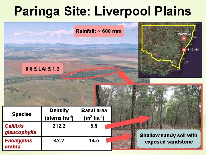
Paringa Site: Liverpool Plains Rainfall: ~ 600 mm PARINGA SYDNEY 0. 8 ≤ LAI ≤ 1. 2 Density (stems ha-1) Basal area (m 2 ha-1) Callitris glaucophylla 212. 2 5. 9 Eucalyptus crebra 42. 2 Species 14. 5 Shallow sandy soil with exposed sandstone

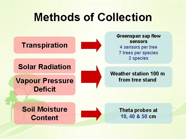
Methods of Collection Transpiration Solar Radiation Vapour Pressure Deficit Soil Moisture Content Greenspan sap flow sensors 4 sensors per tree 7 trees per species 2 species Weather station 100 m from tree stand Theta probes at 10, 40 & 50 cm

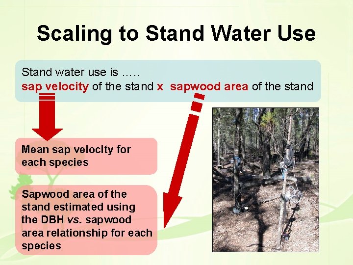
Scaling to Stand Water Use Stand water use is …. . sap velocity of the stand x sapwood area of the stand Mean sap velocity for each species Sapwood area of the stand estimated using the DBH vs. sapwood area relationship for each species

Measurement Time Series

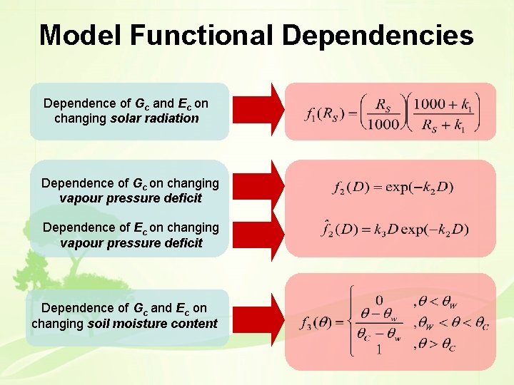
Model Functional Dependencies Dependence of Gc and Ec on changing solar radiation Dependence of Gc on changing vapour pressure deficit Dependence of Ec on changing vapour pressure deficit Dependence of Gc and Ec on changing soil moisture content

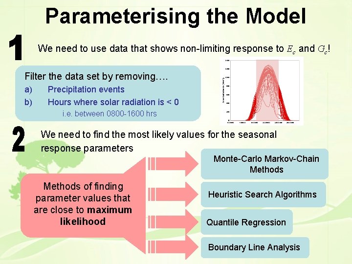
Parameterising the Model We need to use data that shows non-limiting response to Ec and Gc! Filter the data set by removing…. a) b) Precipitation events Hours where solar radiation is < 0 i. e. between 0800 -1600 hrs We need to find the most likely values for the seasonal response parameters Monte-Carlo Markov-Chain Methods of finding parameter values that are close to maximum likelihood Heuristic Search Algorithms Quantile Regression Boundary Line Analysis

Jarvis-Stewart Model: for Gc: Jarvis-Stewart Model: for Ec Functional Relationships

Summer Winter

Residuals and Correlation

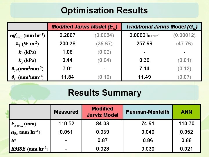
Optimisation Results Modified Jarvis Model (Ec ) Traditional Jarvis Model (Gc ) refmax (mm hr-1) 0. 2667 (0. 0054) 0. 00821 mm s-1 (0. 00012) k 1 (W m-2) 200. 38 (39. 67) 257. 99 (47. 76) k 2 (k. Pa) 1. 08 (0. 02) - - k 3 (k. Pa) 0. 44 (0. 04) 0. 39 (0. 01) θW (mm 3 mm-3) 7. 0* - 7. 14 (0. 12) θC (mm 3 mm-3) 11. 84 (0. 10) 11. 49 (0. 07) Results Summary Measured Modified Jarvis Model Penman-Monteith ANN Ec total (mm) 110. 52 84. 03 74. 91 110. 70 μEc (mm hr-1) 0. 051 0. 039 0. 040 0. 052 R 2 - 0. 87 0. 86 RMSE (mm hr-1) - 0. 028 0. 030 0. 021

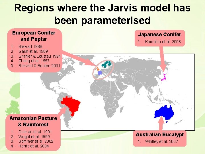
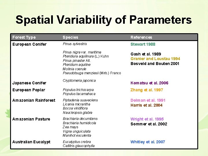
Regions where the Jarvis model has been parameterised European Conifer and Poplar 1. 2. 3. 4. 5. Japanese Conifer 1. Komatsu et al. 2006 Stewart 1988 Gash et al. 1989 Granier & Loustau 1994 Zhang et al. 1997 Bosveld & Bouten 2001 Amazonian Pasture & Rainforest 1. 2. 3. 4. Dolman et al. 1991 Wright et al. 1995 Sommer et al. 2002 Harris et al. 2004 Australian Eucalypt 1. Whitley et al. 2007

Spatial Variability of Parameters

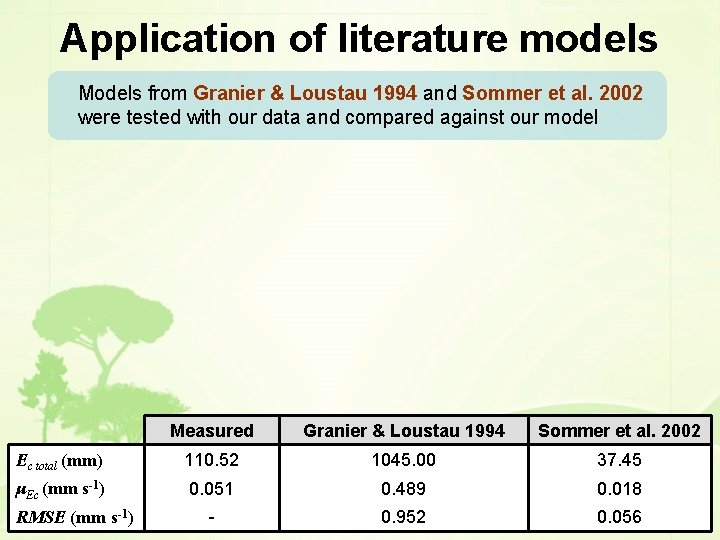
Application of literature models Models from Granier & Loustau 1994 and Sommer et al. 2002 were tested with our data and compared against our model Measured Granier & Loustau 1994 Sommer et al. 2002 Ec total (mm) 110. 52 1045. 00 37. 45 μEc (mm s-1) 0. 051 0. 489 0. 018 - 0. 952 0. 056 RMSE (mm s-1)

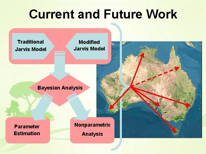
Current and Future Work Traditional Jarvis Model Modified Jarvis Model Bayesian Analysis Parameter Estimation Nonparametric Analysis

Acknowledgements Many thanks to Gab Abramowitz for lending his code and his help with SOLO. and the lab team at UTS for the data

Thank you for your time

Extra Slides

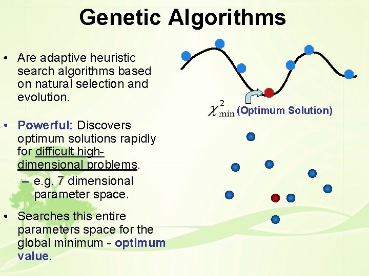
Genetic Algorithms • Are adaptive heuristic search algorithms based on natural selection and evolution. (Optimum Solution) • Powerful: Discovers optimum solutions rapidly for difficult highdimensional problems. – e. g. 7 dimensional parameter space. • Searches this entire parameters space for the global minimum - optimum value.

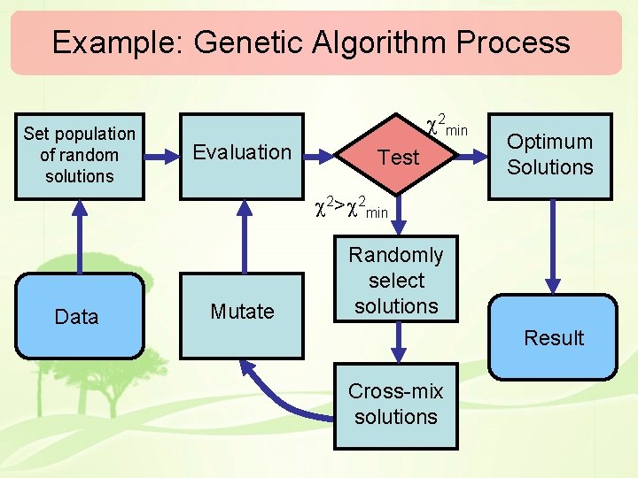
Example: Genetic Algorithm Process Set population of random solutions 2 min Evaluation Test Optimum Solutions 2> 2 min Data Mutate Randomly select solutions Result Cross-mix solutions

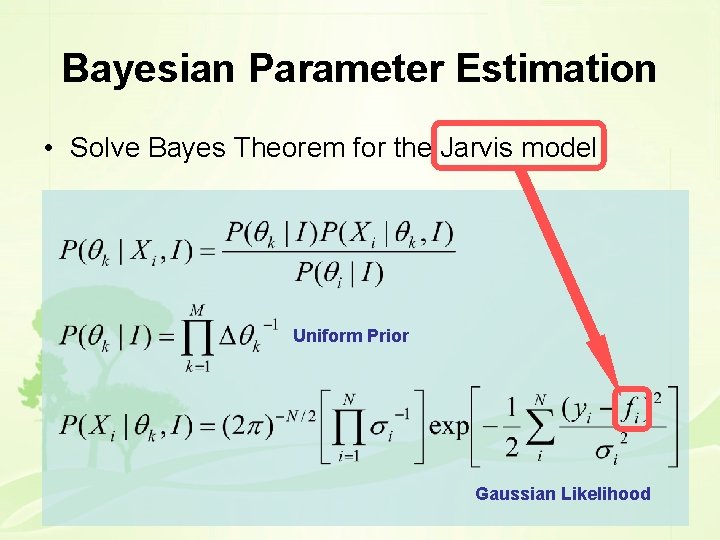
Bayesian Parameter Estimation • Solve Bayes Theorem for the Jarvis model Uniform Prior Gaussian Likelihood

Spatial Variability of Parameters Forest Type Species References European Conifer Pinus sylvestris Stewart 1988 Pinus nigra var. maritima Pteridiura aquilinura (L. ) Kuhn Pinus pinaster Ait. Pteridium aquiline Molinia coerule Pseudotsuga menziesii (Mirb. ) Franco Gash et al. 1989 Granier and Loustau 1994 Bosveld and Bouten 2001 Japanese Conifer Cryptomeria japonica Komatsu et al. 2006 European Poplar Populus trichocarpa Populus tacamahaca Zhang et al. 1997 Amazonian Rainforest Piptadenia suaveolens Licania micrantha Bocoa viridiflora Naucleopsis glabra Dolman et al. 1991 Harris et al. 2004 Amazonian Pasture Brachiaria decumbens Brachiaria humidicola Zea mays Vigna unguiculata Manihot esculenta Wright et al. 1995 Sommer et al. 2002 Australian Eucalyptus crebra Callitris glaucophylla Whitley et al. 2007

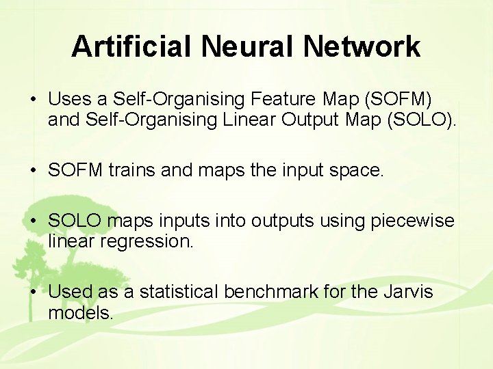
Artificial Neural Network • Uses a Self-Organising Feature Map (SOFM) and Self-Organising Linear Output Map (SOLO). • SOFM trains and maps the input space. • SOLO maps inputs into outputs using piecewise linear regression. • Used as a statistical benchmark for the Jarvis models.

Architecture of SOLO SOFM Network Input Classification Map wji I/O Prediction Map 1. 0 x 1 x 2 xn zj vji Linear Mapping Network

Setup of Models Jarvis-Stewart Model For Gc: Jarvis-Stewart Model For Ec: