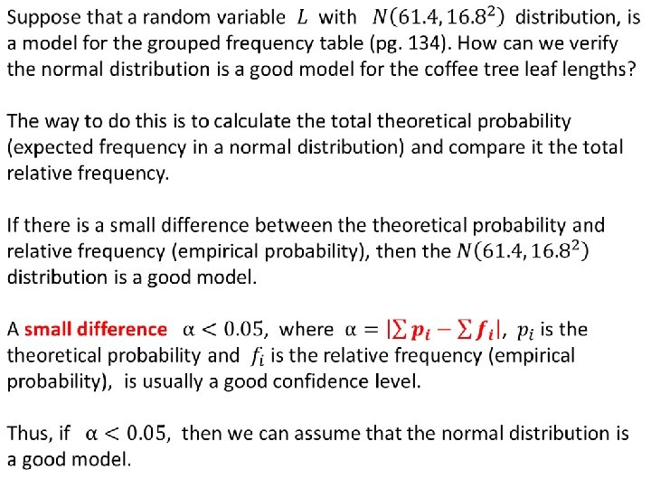
Modeling with the normal distribution The normal distribution

Modeling with the normal distribution The normal distribution is often used as a model for practical situations. In the example that follows, you need to translate the given information into the language of the normal distribution in order to solve the problem.

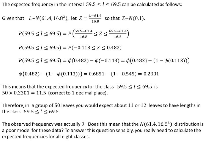
Relative Class Relative frequency Length (mm) f Frequency Boundaries Width density 30 -39 3 0. 060 29. 5 -39. 5 10 0. 006 40 -49 9 0. 180 39. 5 -49. 5 10 0. 018 50 -59 15 0. 300 49. 5 -59. 5 10 0. 030 60 -69 9 0. 180 59. 5 -69. 5 10 0. 018 70 -79 6 0. 120 69. 5 -79. 5 10 0. 012 80 -89 4 0. 080 79. 5 -89. 5 10 0. 008 90 -99 3 0. 060 89. 5 -99. 5 10 0. 006 100 -109 1 0. 020 99. 5 -109. 5 10 0. 002 Total: 50. 000 1. 000

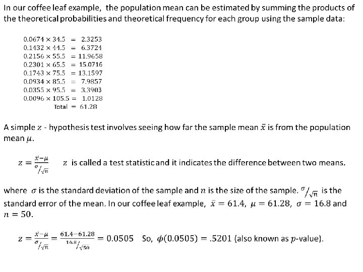
1 1 2 1 1 1 2 2 2 2 1 5 1 2 2 2 2 31. 000 34. 000 39. 000 40. 000 42. 000 43. 000 44. 000 46. 000 47. 000 48. 000 50. 000 52. 000 53. 000 54. 000 56. 000 57. 000 58. 000 60. 000 63. 000 66. 000 67. 000 68. 000 70. 000 72. 000 0. 020 0. 040 0. 020 0. 100 0. 020 0. 040 0. 62 0. 68 0. 78 0. 8 1. 68 0. 86 0. 88 0. 92 1. 88 0. 96 2 2. 08 2. 12 2. 16 1. 12 5. 7 1. 16 2. 4 2. 52 1. 32 2. 68 2. 72 2. 88 961. 000 1156. 000 1521. 000 1600. 000 1764. 000 1849. 000 1936. 000 2116. 000 2209. 000 2304. 000 2500. 000 2704. 000 2809. 000 2916. 000 3136. 000 3249. 000 3364. 000 3600. 000 3969. 000 4356. 000 4489. 000 4624. 000 4900. 000 5184. 000 19. 22 23. 12 30. 42 32 70. 56 36. 98 38. 72 42. 32 88. 36 46. 08 100 108. 16 112. 36 116. 64 62. 72 324. 9 67. 28 144 158. 76 87. 12 179. 56 184. 96 196 207. 36

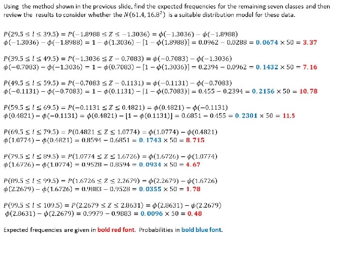
Observed Relative Freq. Theoretical Frequency Empirical Prob. Frequency Probability 3 0. 06 3 or 4 0. 0674 9 0. 18 7 or 8 0. 1432 15 0. 30 10 or 11 0. 2156 9 0. 18 11 or 12 0. 2301 6 0. 12 8 or 9 0. 1743 4 0. 08 4 or 5 0. 0934 3 0. 06 1 or 2 0. 0355 1 0. 02 0 or 1 0. 0096 50 1. 00 0. 97

Now do Exercise 9 C.