MODELING VOLATILITY BY ARCHGARCH MODELS 1 VARIANCE A

MODELING VOLATILITY BY ARCHGARCH MODELS 1

VARIANCE • A time series is said to be heteroscedastic, if its variance changes over time, otherwise it is called homoscedastic. • When the variance is not constant ( it will follow mixture normal distribution), we can expect more outliers than expected from normal distribution. i. e. when a process is heteroscedastic, it will follow heavy-tailed or outlier-prone probability distributions. 2

VARIANCE • Until the early 80 s econometrics had focused almost solely on modeling the means of series, i. e. their actual values. Recently however researchers have focused increasingly on the importance of volatility, its determinates and its effects on mean values. • A key distinction is between the conditional and unconditional variance. • The unconditional variance is just the standard measure of the variance Var(X) =E(X E(X))2 3

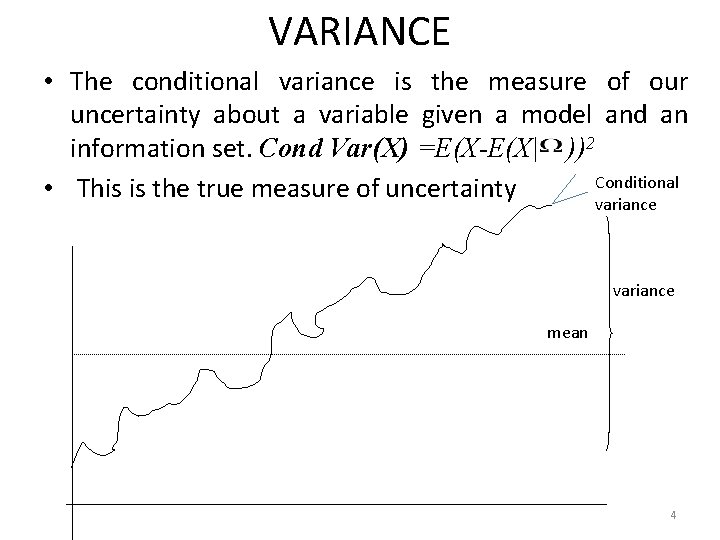
VARIANCE • The conditional variance is the measure of our uncertainty about a variable given a model and an information set. Cond Var(X) =E(X-E(X| ))2 Conditional • This is the true measure of uncertainty variance mean 4

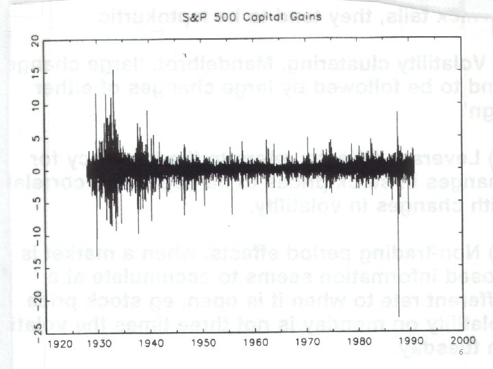
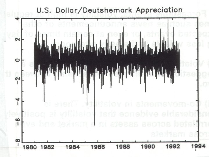
VARIANCE • Stylized Facts of asset returns i. ii. Thick tails: they tend to be leptokurtic Volatility clustering: Mandelbrot, “large changes tend to be followed by large changes of either sign” iii. Leverage Effects: the tendency for changes in stock prices to be negatively correlated with changes in volatility. iv. Non-trading period effects: when a market is closed, information seems to accumulate at a different rate to when it is open. e. g. stock price volatility on Monday is not three times the volatility on Tuesday. v. Forecastable events: volatility is high at regular times such as news announcements or other expected events, or even at certain times of day, e. g. less volatile in the early afternoon. vi. Volatility and serial correlation: There is a suggestion of an inverse relationship between the two. vii. Co-movements in volatility: There is considerable evidence that volatility is positively correlated across assets in a market and even across markets 5

6

7

ARCH MODEL • Stock market’s volatility is rarely constant over time. • In finance, portfolios of financial assets are held as functions of the expected mean and variance of the rate of return. Since any shift in asset demand must be associated with changes in expected mean and variance of rate of return, ARCH models are the best suitable models. • In regression, ARCH models can be used to approximate the complex models. 8

ARCH MODEL • Even though the errors may be serially uncorrelated they are not independent, there will be volatility clustering and fat tails. • If there is no serial correlation of the series but there is of the squared series, then we will say there is weak dependence. This will lead us to examine the volatility of the series, since that is demonstrated by the squared terms. 9

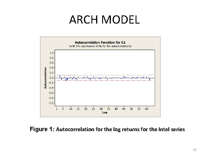
ARCH MODEL Figure 1: Autocorrelation for the log returns for the Intel series 10

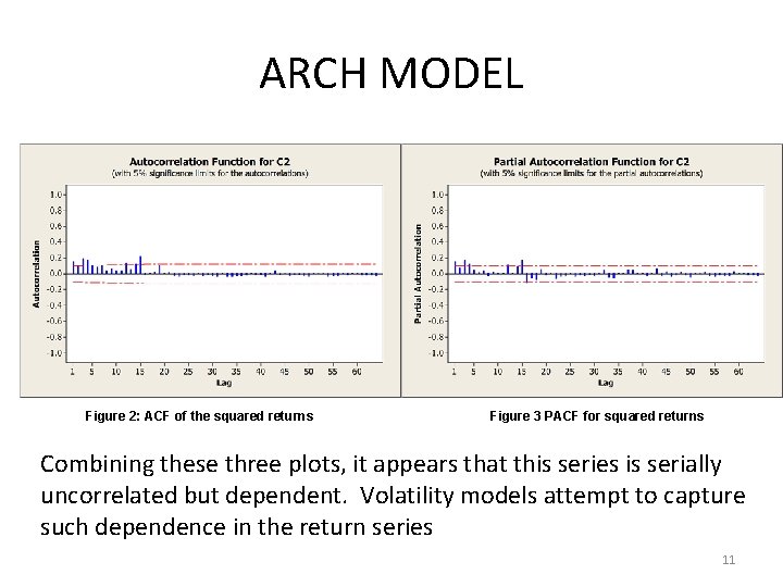
ARCH MODEL Figure 2: ACF of the squared returns Figure 3 PACF for squared returns Combining these three plots, it appears that this series is serially uncorrelated but dependent. Volatility models attempt to capture such dependence in the return series 11

ARCH MODEL • Engle(1982) introduced a model in which the variance at time t is modeled as a linear combination of past squared residuals and called it an ARCH (autoregressive conditionally heteroscedastic) process. • Bolerslev (1986) introduced a more general structure in which the variance model looks more like an ARMA than an AR and called this a GARCH (generalized ARCH) process. 12

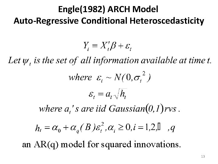
Engle(1982) ARCH Model Auto-Regressive Conditional Heteroscedasticity an AR(q) model for squared innovations. 13

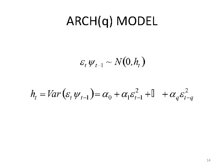
ARCH(q) MODEL 14

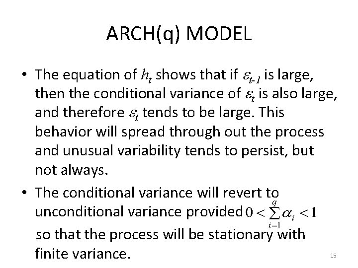
ARCH(q) MODEL • The equation of ht shows that if t-1 is large, then the conditional variance of t is also large, and therefore t tends to be large. This behavior will spread through out the process and unusual variability tends to persist, but not always. • The conditional variance will revert to unconditional variance provided so that the process will be stationary with finite variance. 15

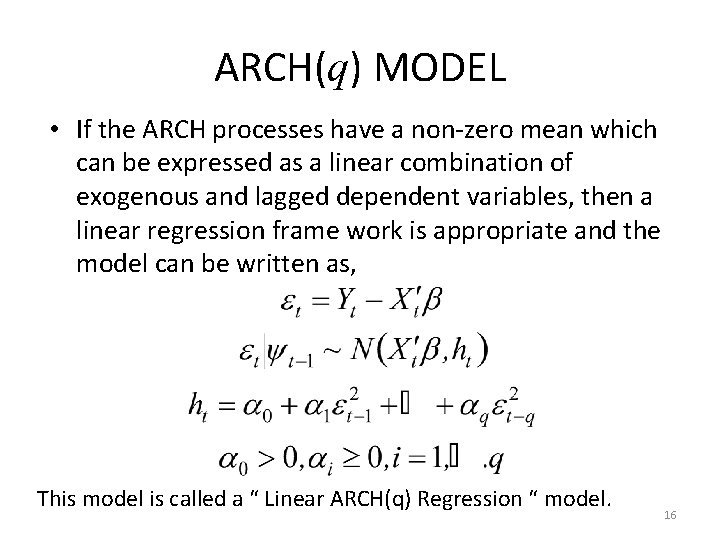
ARCH(q) MODEL • If the ARCH processes have a non-zero mean which can be expressed as a linear combination of exogenous and lagged dependent variables, then a linear regression frame work is appropriate and the model can be written as, This model is called a “ Linear ARCH(q) Regression “ model. 16

ARCH(q) • If the regressors include no lagged dependent variables and can be treated as fixed constants then the ordinary least square (OLS) estimator is the best linear unbiased estimator for the model. However, maximum-likelihood estimator is nonlinear and is more efficient than OLS estimator. 17

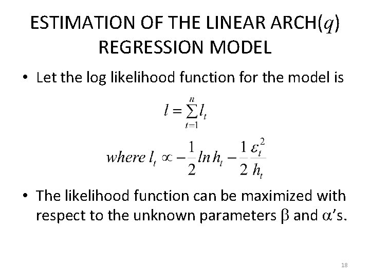
ESTIMATION OF THE LINEAR ARCH(q) REGRESSION MODEL • Let the log likelihood function for the model is • The likelihood function can be maximized with respect to the unknown parameters and ’s. 18

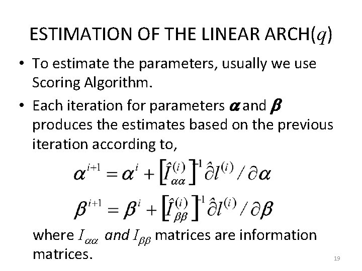
ESTIMATION OF THE LINEAR ARCH(q) • To estimate the parameters, usually we use Scoring Algorithm. • Each iteration for parameters and produces the estimates based on the previous iteration according to, where I and I matrices are information matrices. 19

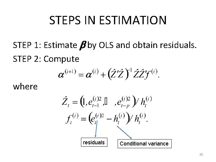
STEPS IN ESTIMATION STEP 1: Estimate by OLS and obtain residuals. STEP 2: Compute where residuals Conditional variance 20

STEPS IN ESTIMATION STEP 3: Using (i+1), compute 21

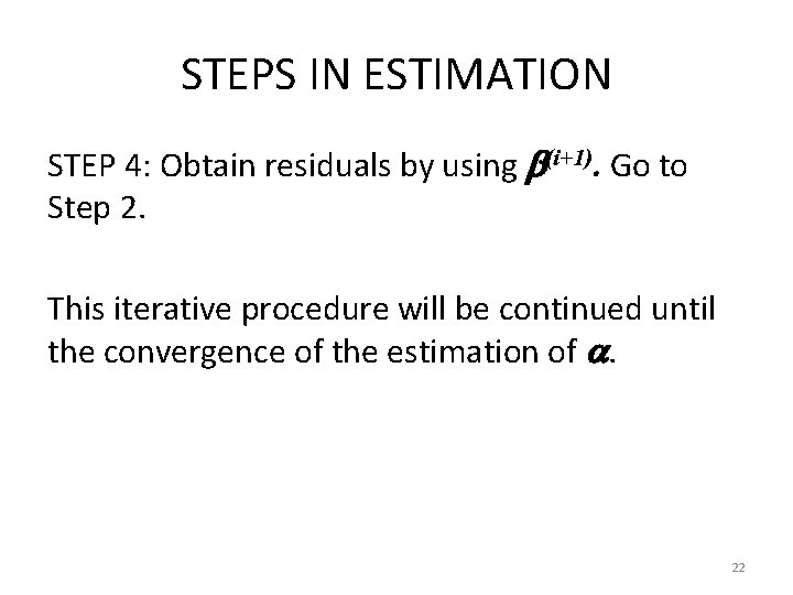
STEPS IN ESTIMATION STEP 4: Obtain residuals by using (i+1). Go to Step 2. This iterative procedure will be continued until the convergence of the estimation of . 22

TESTING FOR ARCH DISTURBANCES • Method 1. The autocorrelation structure of residuals and the squared residuals can be examined. An indication of ARCH is that the residuals will be uncorrelated but the squared residuals will show autocorrelation. 23

TESTING FOR ARCH DISTURBANCES • Method 2. A test based on Lagrange Multiplier ( LM ) principle can be applied. Consider the null hypothesis of no ARCH errors versus the alternative hypothesis that the conditional error variance is given by an ARCH(q) process. The test approach proposed by Engle is to regress the squared residuals on a constant and q lagged residuals. From the residuals of this auxiliary regression, a test statistic is calculated as n. R 2, where R 2 is coming from the auxiliary regression. The null hypothesis will be rejected if the test statistic exceeds the critical value from a chi-square distribution with q degree of freedom. 24

PROBLEMS IN ARCH MODELING • In most of the applications of the ARCH model a relatively long lag in the conditional variance is often called for, and this leads to the problem of negative variance and non-stationarity. To avoid this problem, generally a fixed lag structure is typically imposed. So it is necessary to extent the ARCH models to a new class of models allowing for a both long memory and much more flexible lag structure. • Bollerslev introduced a Generalized ARCH (GARCH) models which allows long memory and flexible lag structure. 25

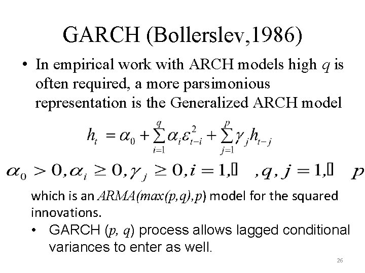
GARCH (Bollerslev, 1986) • In empirical work with ARCH models high q is often required, a more parsimonious representation is the Generalized ARCH model which is an ARMA(max(p, q), p) model for the squared innovations. • GARCH (p, q) process allows lagged conditional variances to enter as well. 26

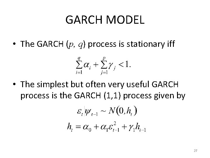
GARCH MODEL • The GARCH (p, q) process is stationary iff • The simplest but often very useful GARCH process is the GARCH (1, 1) process given by 27

TESTING FOR GARCH DISTURBANCES • METHOD 1: Use the previous LM test for ARCH. If the null hypothesis is rejected for long disturbances, GARCH model is appropriate. • METHOD 2: A test based on Lagrange Multiplier (LM) principle can be applied. Consider the null hypothesis of ARCH (q) for errors versus the alternative hypothesis that the errors are given by a GARCH (p, q) process. 28

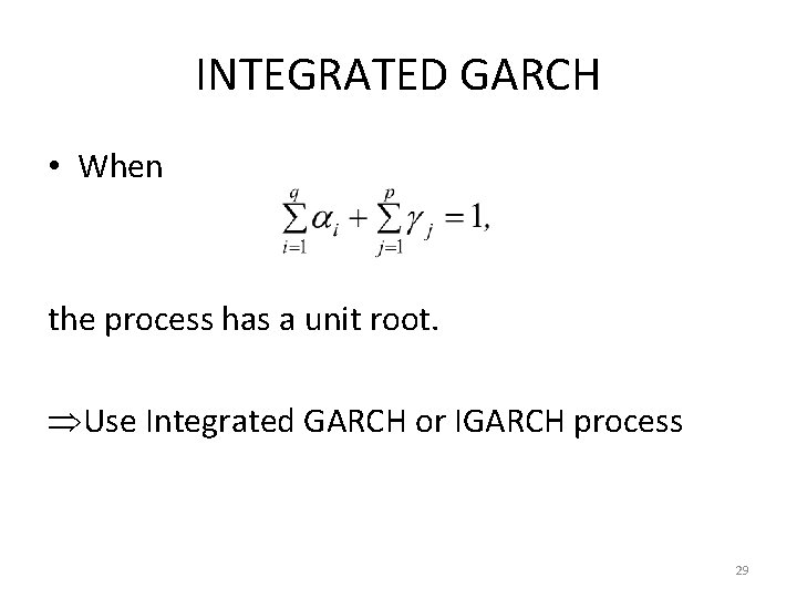
INTEGRATED GARCH • When the process has a unit root. Use Integrated GARCH or IGARCH process 29

SYMMETRYCITY OF GARCH MODELS • In ARCH, GARCH, IGARCH processes, the effect of errors on the conditional variance is symmetric, i. e. , positive error has the same effect as a negative error. • However, in finance, good and bad news have different effects on the volatility. • Positive shock has a smaller effect than the negative shock of the same magnitude. 30

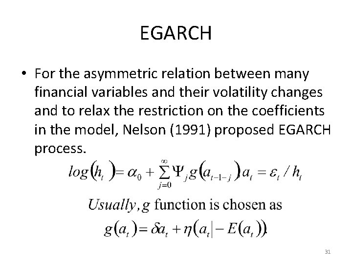
EGARCH • For the asymmetric relation between many financial variables and their volatility changes and to relax the restriction on the coefficients in the model, Nelson (1991) proposed EGARCH process. 31

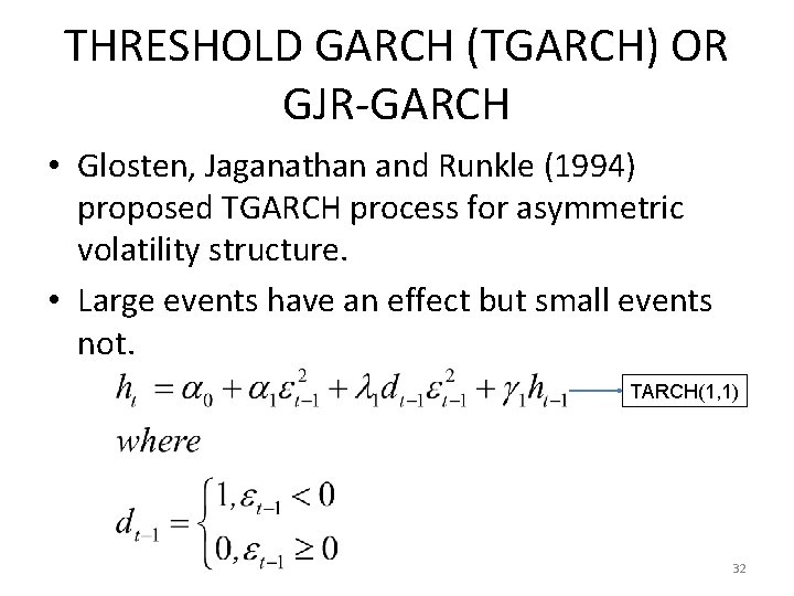
THRESHOLD GARCH (TGARCH) OR GJR-GARCH • Glosten, Jaganathan and Runkle (1994) proposed TGARCH process for asymmetric volatility structure. • Large events have an effect but small events not. TARCH(1, 1) 32

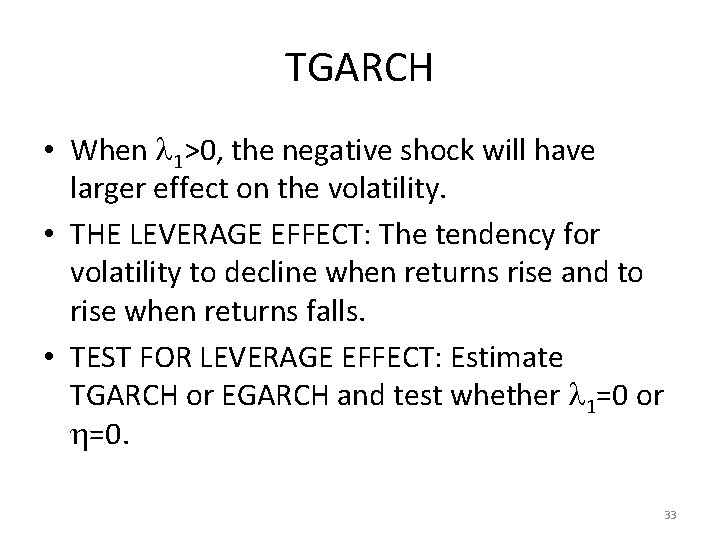
TGARCH • When 1>0, the negative shock will have larger effect on the volatility. • THE LEVERAGE EFFECT: The tendency for volatility to decline when returns rise and to rise when returns falls. • TEST FOR LEVERAGE EFFECT: Estimate TGARCH or EGARCH and test whether 1=0 or =0. 33

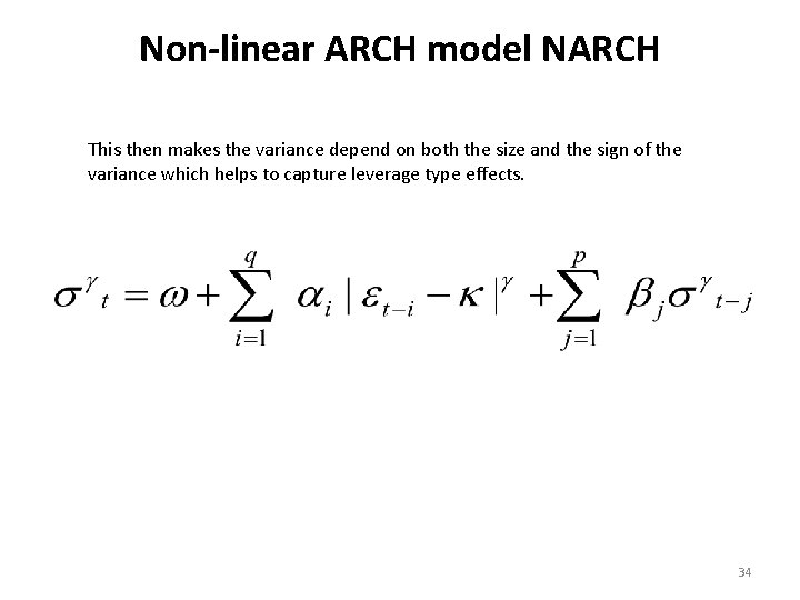
Non-linear ARCH model NARCH This then makes the variance depend on both the size and the sign of the variance which helps to capture leverage type effects. 34

ARCH in MEAN (G)ARCH-M Many classic areas of finance suggest that the mean of a relationship will be affected by the volatility or uncertainty of a series. Engle Lilien and Robins(1987) allow for this explicitly using an ARCH framework. typically either the variance or the standard deviation are included in the mean relationship. 35

Non normality assumptions While the basic GARCH model allows a certain amount of leptokurtic behaviour, this is often insufficient to explain real world data. Some authors therefore assume a range of distributions other than normality which help to allow for the fat tails in the distribution. t Distribution The t distribution has a degrees of freedom parameter which allows greater kurtosis. 36

THE GARCH ZOO • QARCH = quadratic ARCH • TARCH = threshold ARCH • STARCH = structural ARCH • SWARCH = switching ARCH • QTARCH = quantitative threshold ARCH • vector ARCH • diagonal ARCH • factor ARCH 37

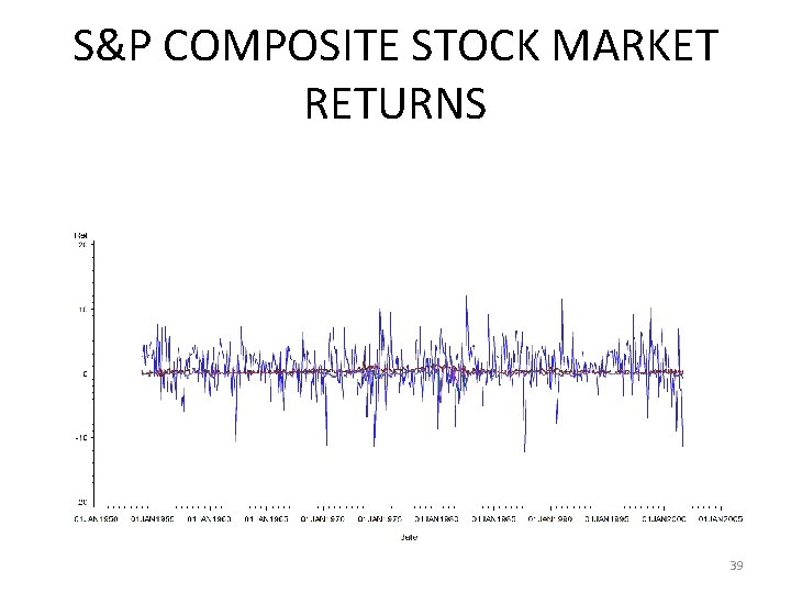
S&P COMPOSITE STOCK MARKET RETURNS • Monthly data on the S&P Composite index returns over the period 1954: 1– 2001: 9. Lags of the inflation rate and the change in the three-month Treasury bill (T-bill) rate are used as regressors, in addition to lags of the returns. We begin by modeling the returns series as a function of a constant, one lag of returns (Ret_l), one lag of the inflation rate (Inf_l) and one lag of the first-difference of the three-month T-bill rate (DT-bill_l). 38

S&P COMPOSITE STOCK MARKET RETURNS 39

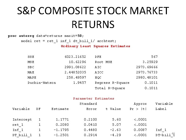
S&P COMPOSITE STOCK MARKET RETURNS proc autoreg data=returns maxit=50; model ret = ret_1 inf_1 dt_bill_1/ archtest; Ordinary Least Squares Estimates SSE MSE SBC MAE MAPE Durbin-Watson Variable Intercept ret_1 Inf_1 DT_bill_1 6023. 21652 10. 62296 2991. 08622 2. 44852035 258. 49597 1. 9457 DF Estimate 1 1 1. 1771 0. 2080 -1. 1795 -1. 2501 DFE Root MSE AICC HQC Regress R-Square Total R-Square Parameter Estimates Standard Error t Value 0. 2100 0. 0410 0. 4480 0. 2914 5. 60 5. 07 -2. 63 -4. 29 567 3. 25929 2973. 69666 2973. 76733 2980. 48101 0. 1011 Approx Pr > |t| <. 0001 0. 0087 <. 0001 Variable Label Inf_1 40 DT-bill_1

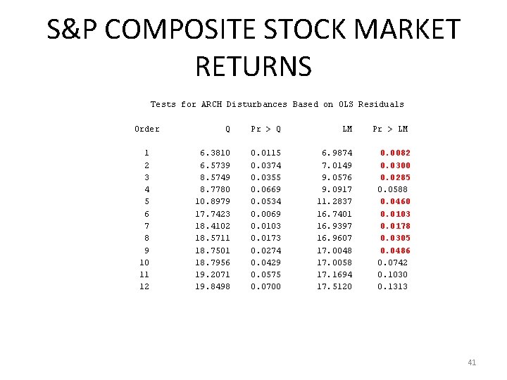
S&P COMPOSITE STOCK MARKET RETURNS Tests for ARCH Disturbances Based on OLS Residuals Order 1 2 3 4 5 6 7 8 9 10 11 12 Q Pr > Q LM Pr > LM 6. 3810 6. 5739 8. 5749 8. 7780 10. 8979 17. 7423 18. 4102 18. 5711 18. 7501 18. 7956 19. 2071 19. 8498 0. 0115 0. 0374 0. 0355 0. 0669 0. 0534 0. 0069 0. 0103 0. 0173 0. 0274 0. 0429 0. 0575 0. 0700 6. 9874 7. 0149 9. 0576 9. 0917 11. 2837 16. 7401 16. 9397 16. 9607 17. 0048 17. 0058 17. 1694 17. 5120 0. 0082 0. 0300 0. 0285 0. 0588 0. 0460 0. 0103 0. 0178 0. 0305 0. 0486 0. 0742 0. 1030 0. 1313 41

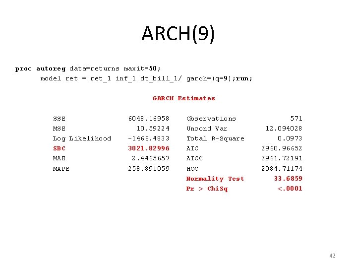
ARCH(9) proc autoreg data=returns maxit=50; model ret = ret_1 inf_1 dt_bill_1/ garch=(q=9); run; GARCH Estimates SSE MSE Log Likelihood SBC MAE MAPE 6048. 16958 10. 59224 -1466. 4833 3021. 82996 2. 4465657 258. 891059 Observations Uncond Var Total R-Square AICC HQC Normality Test Pr > Chi. Sq 571 12. 094028 0. 0973 2960. 96652 2961. 72191 2984. 71174 33. 6859 <. 0001 42

ARCH(9) Parameter Estimates Variable Intercept ret_1 Inf_1 DT_bill_1 ARCH 0 ARCH 1 ARCH 2 ARCH 3 ARCH 4 ARCH 5 ARCH 6 ARCH 7 ARCH 8 ARCH 9 DF Estimate Standard Error t Value Approx Pr > |t| 1 1. 1960 0. 1897 6. 30 <. 0001 1 0. 2146 0. 0443 4. 84 <. 0001 1 -0. 8773 0. 3807 -2. 30 0. 0212 1 -0. 9640 0. 2491 -3. 87 0. 0001 1 4. 7466 0. 9261 5. 13 <. 0001 1 0. 1207 0. 0477 2. 53 0. 0114 1 0. 005981 0. 0356 0. 17 0. 8667 1 0. 1341 0. 0548 2. 45 0. 0144 1 1. 021 E-19 0 Infty <. 0001 1 0. 1266 0. 0553 2. 29 0. 0220 1 0. 1499 0. 0510 2. 94 0. 0033 1 0. 0179 0. 0402 0. 45 0. 6563 1 -5. 49 E-21 0 -Infty <. 0001 1 0. 0524 0. 0486 1. 08 0. 2812 Variable Label Inf_1 DT-bill_1 43

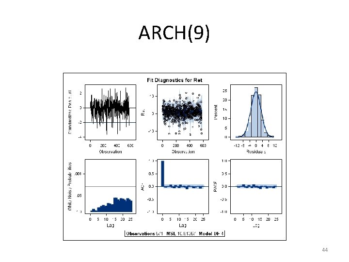
ARCH(9) 44

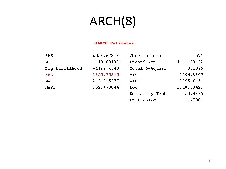
ARCH(8) GARCH Estimates SSE MSE Log Likelihood SBC MAE MAPE 6053. 67303 10. 60188 -1133. 4449 2355. 75315 2. 44715477 259. 470044 Observations Uncond Var Total R-Square AICC HQC Normality Test Pr > Chi. Sq 571 11. 1188142 0. 0965 2294. 8897 2295. 6451 2318. 63492 50. 4365 <. 0001 45

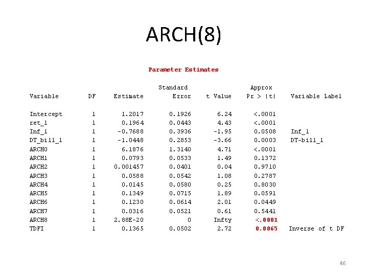
ARCH(8) Parameter Estimates Variable Intercept ret_1 Inf_1 DT_bill_1 ARCH 0 ARCH 1 ARCH 2 ARCH 3 ARCH 4 ARCH 5 ARCH 6 ARCH 7 ARCH 8 TDFI DF Estimate Standard Error 1 1 1 1. 2017 0. 1964 -0. 7688 -1. 0448 6. 1876 0. 0793 0. 001457 0. 0588 0. 0145 0. 1349 0. 1230 0. 0316 2. 88 E-20 0. 1365 0. 1926 0. 0443 0. 3936 0. 2853 1. 3140 0. 0533 0. 0401 0. 0542 0. 0580 0. 0715 0. 0614 0. 0521 0 0. 0502 t Value Approx Pr > |t| 6. 24 4. 43 -1. 95 -3. 66 4. 71 1. 49 0. 04 1. 08 0. 25 1. 89 2. 01 0. 61 Infty 2. 72 <. 0001 0. 0508 0. 0003 <. 0001 0. 1372 0. 9710 0. 2787 0. 8030 0. 0591 0. 0449 0. 5441 <. 0001 0. 0065 Variable Label Inf_1 DT-bill_1 Inverse of t DF 46

ARCH(8) 47

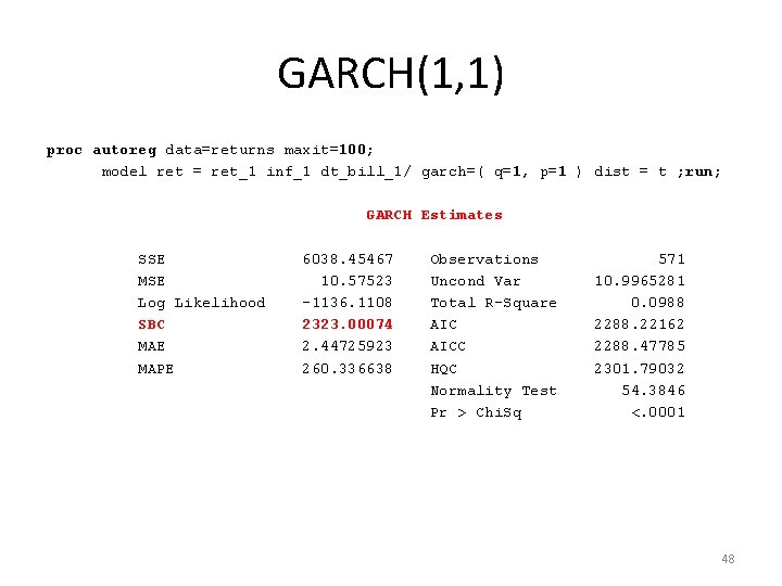
GARCH(1, 1) proc autoreg data=returns maxit=100; model ret = ret_1 inf_1 dt_bill_1/ garch=( q=1, p=1 ) dist = t ; run; GARCH Estimates SSE MSE Log Likelihood SBC MAE MAPE 6038. 45467 10. 57523 -1136. 1108 2323. 00074 2. 44725923 260. 336638 Observations Uncond Var Total R-Square AICC HQC Normality Test Pr > Chi. Sq 571 10. 9965281 0. 0988 2288. 22162 2288. 47785 2301. 79032 54. 3846 <. 0001 48

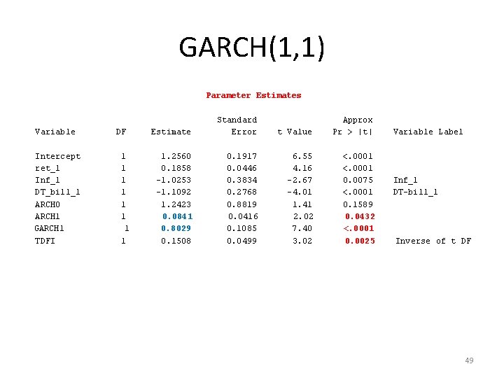
GARCH(1, 1) Parameter Estimates Variable Intercept ret_1 Inf_1 DT_bill_1 ARCH 0 ARCH 1 GARCH 1 TDFI DF 1 1 1 1 Estimate Standard Error t Value Approx Pr > |t| 1. 2560 0. 1858 -1. 0253 -1. 1092 1. 2423 0. 0841 0. 8029 0. 1508 0. 1917 0. 0446 0. 3834 0. 2768 0. 8819 0. 0416 0. 1085 0. 0499 6. 55 4. 16 -2. 67 -4. 01 1. 41 2. 02 7. 40 3. 02 <. 0001 0. 0075 <. 0001 0. 1589 0. 0432 <. 0001 0. 0025 Variable Label Inf_1 DT-bill_1 Inverse of t DF 49

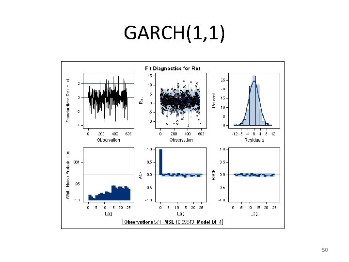
GARCH(1, 1) 50

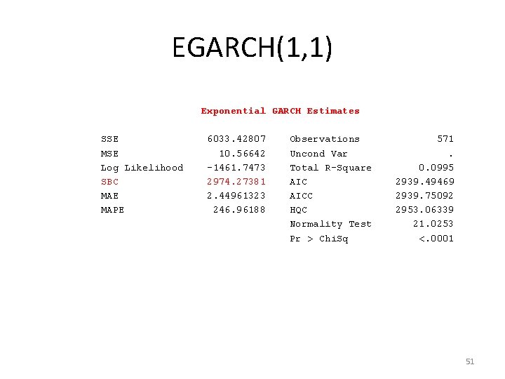
EGARCH(1, 1) Exponential GARCH Estimates SSE MSE Log Likelihood SBC MAE MAPE 6033. 42807 10. 56642 -1461. 7473 2974. 27381 2. 44961323 246. 96188 Observations Uncond Var Total R-Square AICC HQC Normality Test Pr > Chi. Sq 571. 0. 0995 2939. 49469 2939. 75092 2953. 06339 21. 0253 <. 0001 51

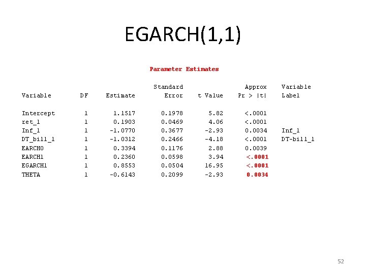
EGARCH(1, 1) Parameter Estimates Variable DF Estimate Standard Error Intercept ret_1 Inf_1 DT_bill_1 EARCH 0 EARCH 1 EGARCH 1 THETA 1 1 1 1 1. 1517 0. 1903 -1. 0770 -1. 0312 0. 3394 0. 2360 0. 8553 -0. 6143 0. 1978 0. 0469 0. 3677 0. 2466 0. 1176 0. 0598 0. 0504 0. 2099 t Value Approx Pr > |t| 5. 82 4. 06 -2. 93 -4. 18 2. 88 3. 94 16. 95 -2. 93 <. 0001 0. 0034 <. 0001 0. 0039 <. 0001 0. 0034 Variable Label Inf_1 DT-bill_1 52

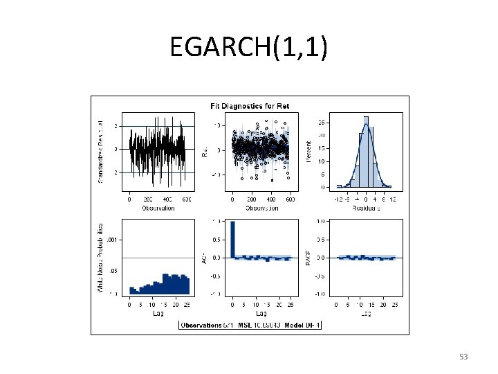
EGARCH(1, 1) 53

IGARCH(1, 1) Integrated GARCH Estimates SSE MSE Log Likelihood SBC MAE MAPE 6034. 97631 10. 56914 -1140. 055 2324. 54181 2. 44746877 259. 845571 Observations Uncond Var Total R-Square AICC HQC Normality Test Pr > Chi. Sq 571 0. 0993 2294. 11008 2294. 30902 2305. 98269 49. 0458 <. 0001 54

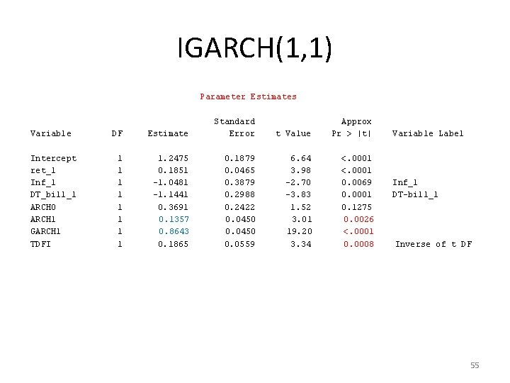
IGARCH(1, 1) Parameter Estimates Variable DF Estimate Standard Error Intercept ret_1 Inf_1 DT_bill_1 ARCH 0 ARCH 1 GARCH 1 TDFI 1 1 1 1 1. 2475 0. 1851 -1. 0481 -1. 1441 0. 3691 0. 1357 0. 8643 0. 1865 0. 1879 0. 0465 0. 3879 0. 2988 0. 2422 0. 0450 0. 0559 t Value Approx Pr > |t| 6. 64 3. 98 -2. 70 -3. 83 1. 52 3. 01 19. 20 3. 34 <. 0001 0. 0069 0. 0001 0. 1275 0. 0026 <. 0001 0. 0008 Variable Label Inf_1 DT-bill_1 Inverse of t DF 55

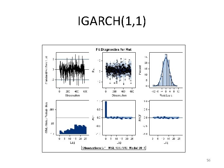
IGARCH(1, 1) 56

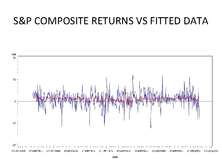
S&P COMPOSITE RETURNS VS FITTED DATA 57

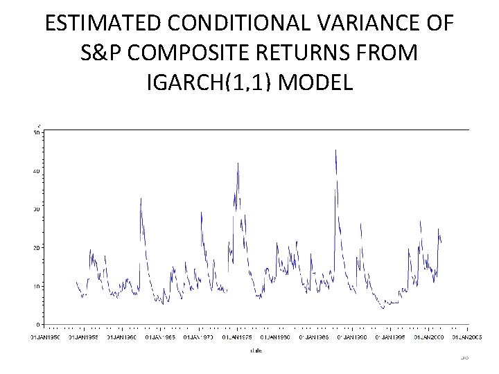
ESTIMATED CONDITIONAL VARIANCE OF S&P COMPOSITE RETURNS FROM IGARCH(1, 1) MODEL 58

REFERENCES • Bollerslev, Tim. 1986. “Generalized Autoregressive Conditional Heteroskedasticity. ” Journal of Econometrics. April, 31: 3, pp. 307– 27. • Engle, Robert F. 1982. “Autoregressive Conditional Heteroskedasticity with Estimates of the Variance of United Kingdom Inflation. ” Econometrica. 50: 4, pp. 987– 1007. • Glosten, Lawrence R. , Ravi Jagannathan and David E. Runkle. 1993. “On the Relation Between the Expected Value and the Volatility of the Nominal Excess Returns on Stocks. ” Journal of Finance. 48: 5, pp. 1779– 801. • Nelson, Daniel B. 1991. “Conditional Heteroscedasticity in Asset Returns: A New Approach. ” Econometrica. 59: 2, pp. 347 – 70. 59