Modeling Uncertainty over time Time series of snapshot

Inference tasks in temporal models • Filtering: posterior distribution over current state given evidence

Uncertainty and Time Hidden Markov Models I p( | ) Emission Probs t P(

Uncertainty and Time Kalman Filtering • Streams of noisy input data • Basic idea

Kalman Filter • Linear Gaussian conditional distributions represent state and sensor models • LG:

Slides: 5

Modeling Uncertainty over time • Time series of snapshot of the world “state” we are interested represented as a set of random variables (RVs) – Observable – Hidden • Stationary process (not static) • Markovian Property (current state depends only on finite history – typically just previous time slice) • Transition Model P(current state/previous state) • Sensor/Observation Model P(evidence/current state) ICASSP 2013 tutorial 1

Inference tasks in temporal models • Filtering: posterior distribution over current state given evidence = likelihood of evidence • Prediction: posterior distribution of future state given evidence to date • Smoothing: posterior distribution of past state given all evidence up to the present • Most likely explanation: given sequence of observations, most likely sequence of states that has generated them • EM-algorithm – Estimate what transitions occurred and what states generated the sensor reading and update models – Updated models provide new estimates and process iterated until convergence ICASSP 2013 tutorial 2

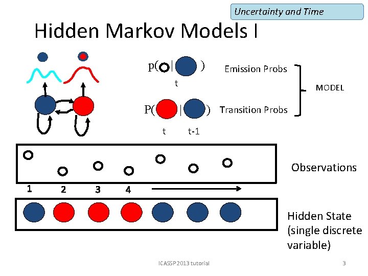
Uncertainty and Time Hidden Markov Models I p( | ) Emission Probs t P( MODEL | t ) Model Transition Probs t-1 Observations 1 2 3 Hidden 4 Hidden State (single discrete Observed variable) ICASSP 2013 tutorial 3

Uncertainty and Time Kalman Filtering • Streams of noisy input data • Basic idea t->t+1 : – Prior knowledge of state – Prediction step (based on some model) – Update step (compare prediction to measurements) – Readjust model – Output estimate of state • Statistically optimal estimate of system state • Particle filters are another approach ICASSP 2013 tutorial 4

Kalman Filter • Linear Gaussian conditional distributions represent state and sensor models • LG: P(x/y)=N(ay y + by, σy)(c) • Next state is linear function of current state plus some Gaussian noise i. e constant dx/dt • Forward step: mean + covariance matrix at t produces mean + covariance matrix at t+1 • Trade-off between observation reliability and model reliability • Variants to relax strong assumptions: switching, extended ICASSP 2013 tutorial 5