Modeling the AtmosOcean System Objectives Climate Models Statistical

Modeling the Atmos-Ocean System Objectives: • Climate Models – Statistical models – 1 D, 2 D models – GCM model • the strengths and weaknesses of GCMs • The application of GCMs 12/22/2021 UNBC 1

• Statistical models: y(t+t’) = F 1(y(t))+F 2(x(t)); (1) If F 1 and F 2 are both linear, the model is linear statistical models. Otherwise models are nonlinear. (2) If F 1=0, models are regression models (3) If F 2=0, models are Markov models. 12/22/2021 UNBC 2

• t’ is the time interval. When t’=0, there is no time ahead for prediction, i. e. , prediction is simultaneous. several common statistical models: (1) Univariate and Multiple Regression (2) Markov models or Auto-Regression (3) Neural Network ………… 12/22/2021 UNBC 3

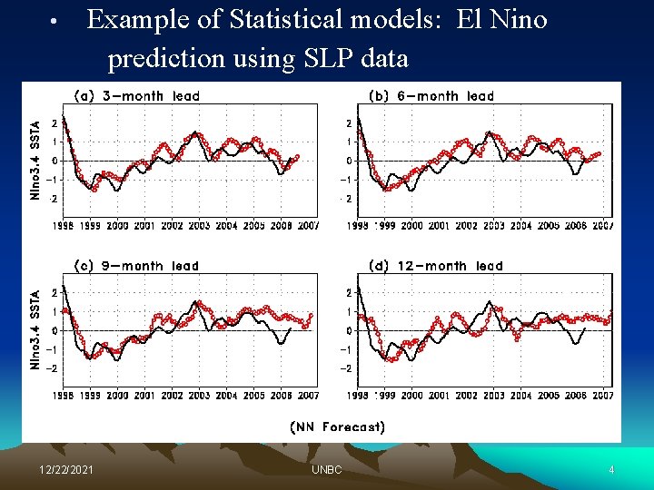
• Example of Statistical models: El Nino prediction using SLP data 12/22/2021 UNBC 4

• Advantage and disadvantages of statistical models: Advantages: simple, cheap and useful. For some problems, statistical models are as good as the most complicated dynamical models. . Disadvantages: (1) need a large of data set, which is often not available. (2) Only statistical, not physical/dynamical (3) statistical relation may shift for different period. 12/22/2021 UNBC 5

• Climate models Use quantitative methods to simulate the interactions of the atmosphere, oceans, land surface, and ice. Climate models are mainly used for predictions and simulations. 12/22/2021 UNBC 6

• Dynamical/physical models Using physical principles to describe the relationship among different components of climate system in the form of mathematical equations. These mathematical equations are called dynamical models. By solving the equations, we can simulate and predict the components of the earth climate system. 12/22/2021 UNBC 7

Climate Model – what does it do? • Starts with known physical laws – conservation of momentum, energy, & mass. • Views atmosphere, oceans, land as a continuum (i. e. all spatial scales present satisfying same laws). • Find and uses numerical approximations to the continuum physical laws. • Integrate in time to develop climate statistics same as observed-evaluate success by extent of agreement. • On global scale, this agenda very successful. 12/22/2021 UNBC 8

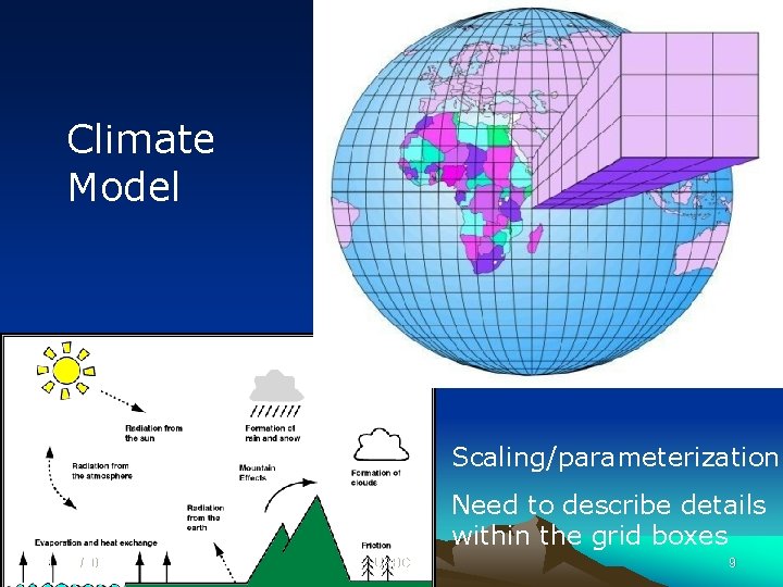
Climate Model Scaling/parameterization Need to describe details within the grid boxes 12/22/2021 UNBC 9

12/22/2021 UNBC 10

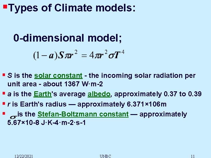
§Types of Climate models: 0 -dimensional model; § S is the solar constant - the incoming solar radiation per unit area - about 1367 W·m-2 § a is the Earth's average albedo, approximately 0. 37 to 0. 39 § r is Earth's radius — approximately 6. 371× 106 m § is the Stefan-Boltzmann constant — approximately 5. 67× 10 -8 J·K-4·m-2·s-1 12/22/2021 UNBC 11

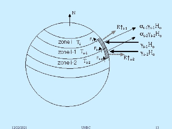
• One dimensional model: The only dimension represented is variation with latitude; atmosphere is averaged vertically and E-W. Multiple processes of N-S heat transport by atmosphere and oceans are usually represented as diffusion. Such models are useful for modeling the interaction of heat transport feedbacks. 12/22/2021 UNBC 12

12/22/2021 UNBC 13

Radiation energy in = Radiation energy out + transport into another zone : 12/22/2021 UNBC 14

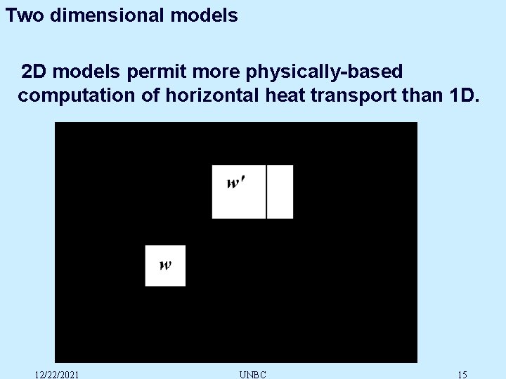
Two dimensional models 2 D models permit more physically-based computation of horizontal heat transport than 1 D. 12/22/2021 UNBC 15

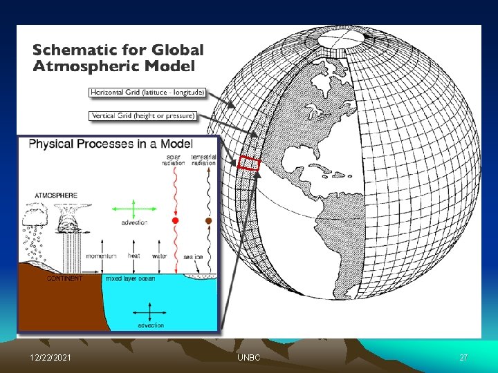
• Global climate model These models are the most complex. The models divide atmosphere or ocean into a horizontal grid with a typical resolution of 2 -4 degree latitude by 2 -4 degree longitude and 10 -20 layers in the vertical. They directly simulate winds, ocean currents and many other processes. Feedback processes are simulated in the coupled atmosphere and ocean GCMs - water vapor, clouds, seasonal snow and ice. 12/22/2021 UNBC 16

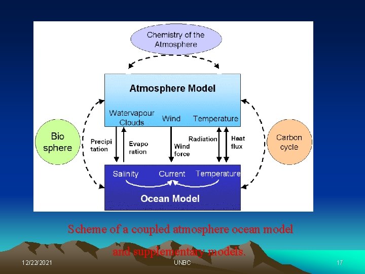
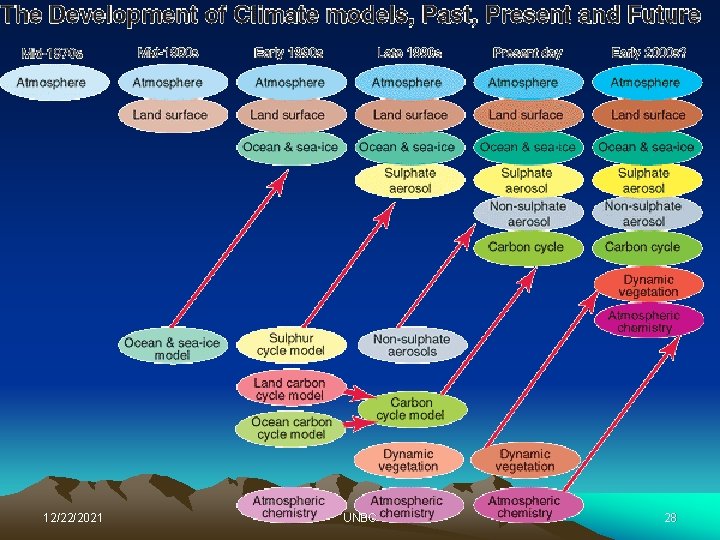
Scheme of a coupled atmosphere ocean model and supplementary models. 12/22/2021 UNBC 17

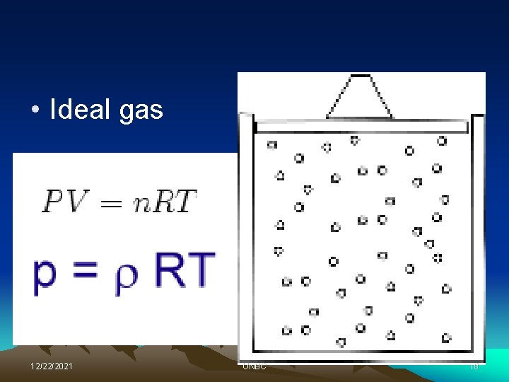
• Ideal gas 12/22/2021 UNBC 18

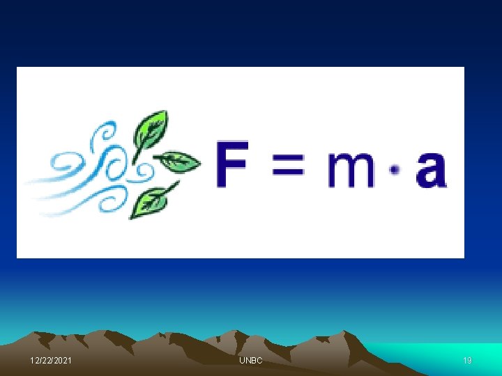
• Newton's law 12/22/2021 UNBC 19

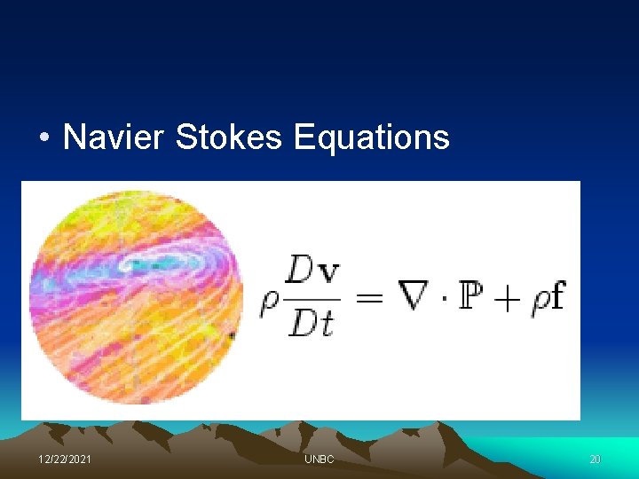
• Navier Stokes Equations 12/22/2021 UNBC 20

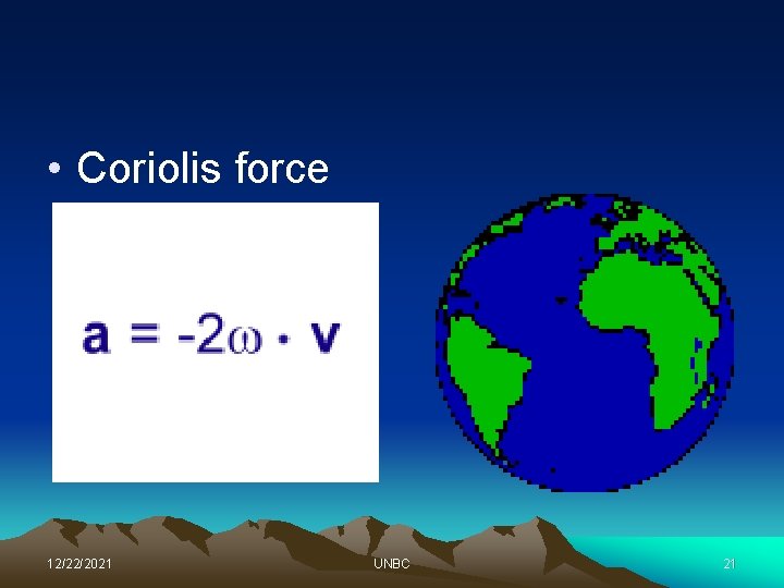
• Coriolis force 12/22/2021 UNBC 21

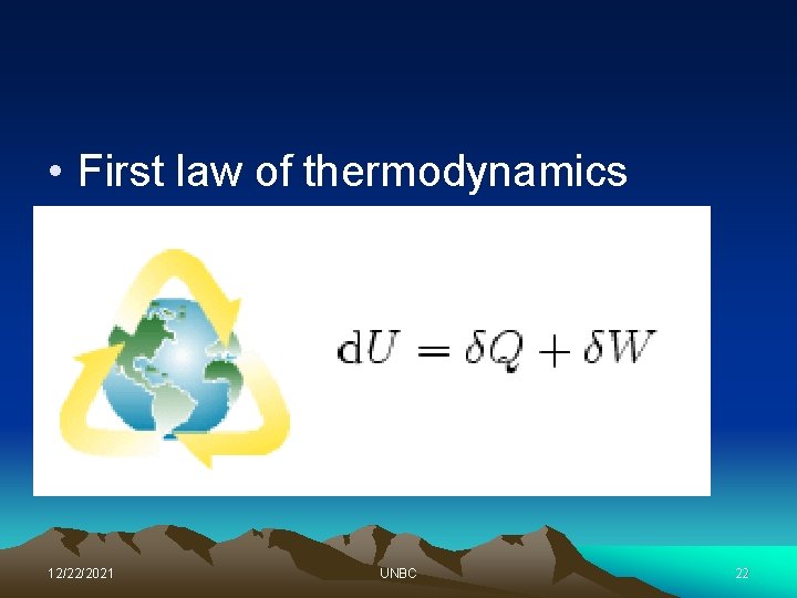
• First law of thermodynamics 12/22/2021 UNBC 22

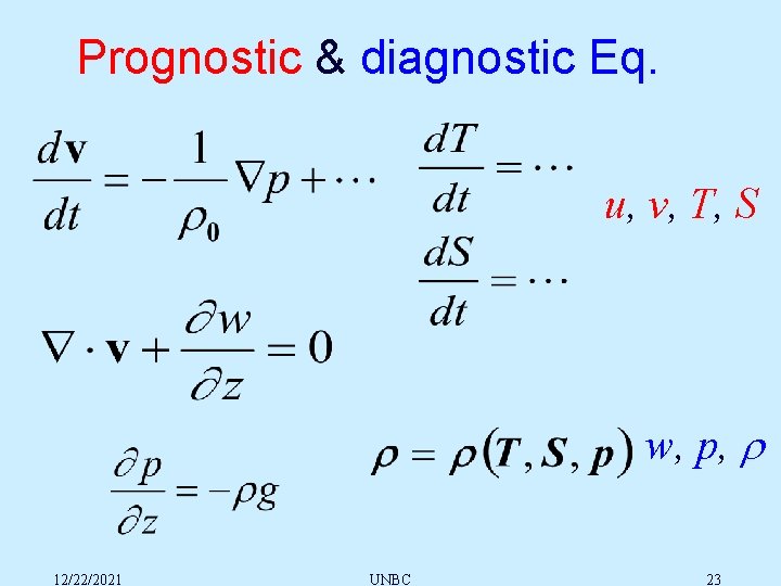
Prognostic & diagnostic Eq. u, v, T, S w, p, 12/22/2021 UNBC 23

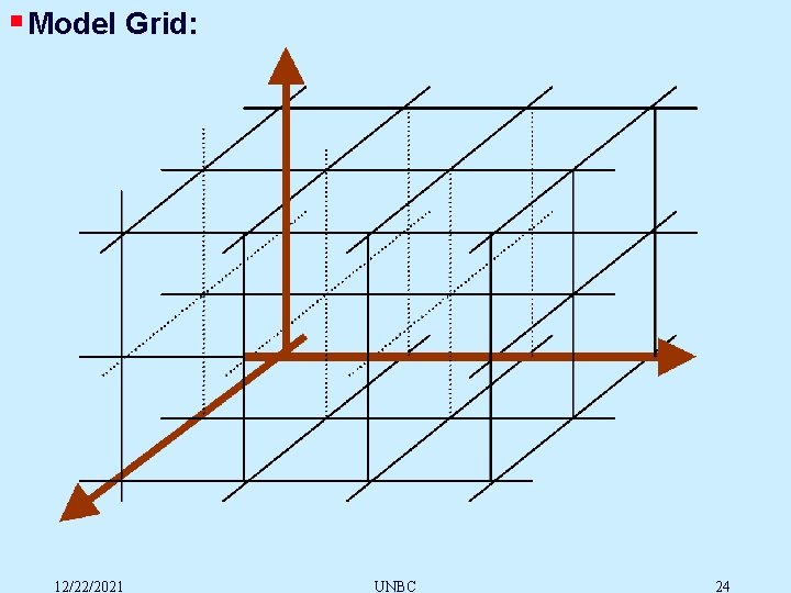
§ Model Grid: 12/22/2021 UNBC 24

• The derivative of a function f at a point x is defined by the limit: Thus, we can use finite differences to approximate derivatives. 12/22/2021 UNBC 25

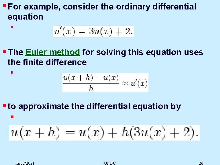
§ For example, consider the ordinary differential equation • § The Euler method for solving this equation uses the finite difference • § to approximate the differential equation by § 12/22/2021 UNBC 26

12/22/2021 UNBC 27

12/22/2021 UNBC 28

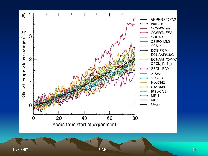
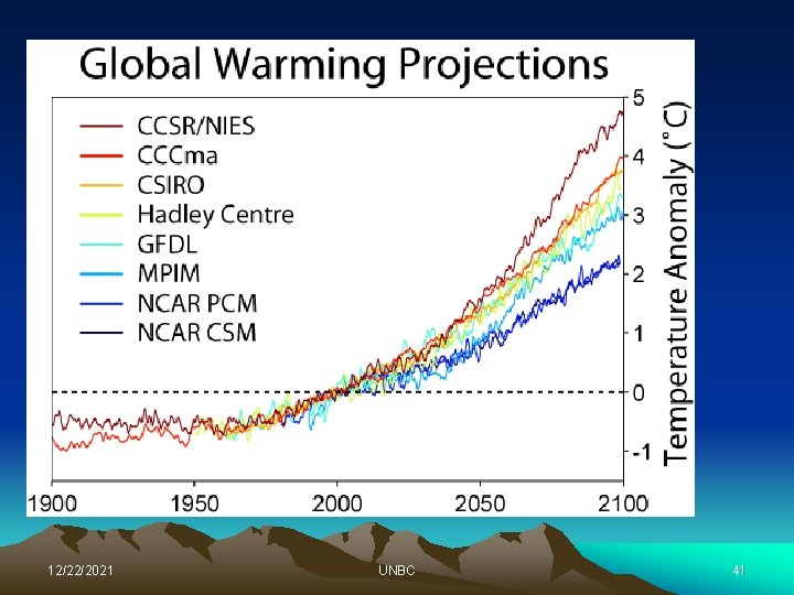
• Projections of future climate change GCMs use a transient climate simulation to project/predict future temperature changes under various scenarios. These can be idealized scenarios (most commonly, CO 2 increasing at 1%/y). 12/22/2021 UNBC 29

• equilibrium climate simulation greenhouse gas concentrations are suddenly changed (typically from pre-industrial values to twice pre-industrial values) and the model allowed to come into equilibrium with the new forcing. • transient climate simulation a mode of running a global climate model in which a period of time (typically 1850 -2100) is simulated with continuously-varying concentrations of greenhouse gases so that the climate of the model represents a realistic mode of possible change in the real world. 12/22/2021 UNBC 30

The Intergovernmental Panel on Climate Change (IPCC) was established in 1988 by two United Nations organizations, the World Meteorological Organization (WMO) and the United Nations Environment Programme (UNEP) to assess the "risk of human-induced climate change". IPCC: first assessment report in 1990 second assessment report in 1995 third assessment report in 2001 fourth assessment report in 2007 12/22/2021 UNBC 31

IPCC reports should be the most authoritative reports on climate change, and are widely cited in almost any debate related to climate change. The reports have been influential in forming national and international responses to climate change. A small but vocal minority (less than 1. 5%) of the scientists involved with the report have accused the IPCC of bias. 12/22/2021 UNBC 32

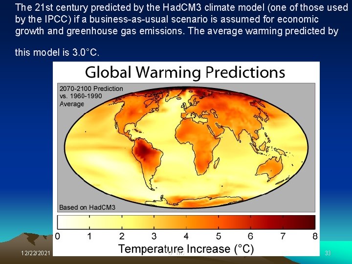
The 21 st century predicted by the Had. CM 3 climate model (one of those used by the IPCC) if a business-as-usual scenario is assumed for economic growth and greenhouse gas emissions. The average warming predicted by this model is 3. 0°C. 12/22/2021 UNBC 33

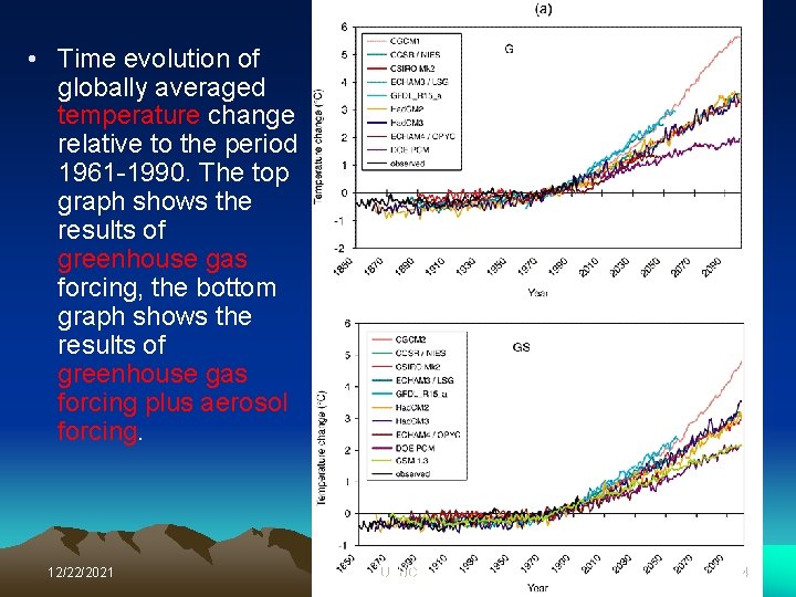
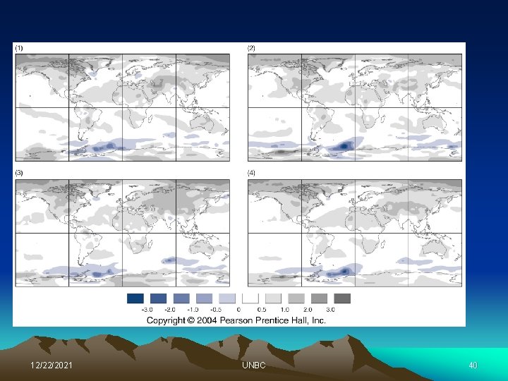
• Time evolution of globally averaged temperature change relative to the period 1961 -1990. The top graph shows the results of greenhouse gas forcing, the bottom graph shows the results of greenhouse gas forcing plus aerosol forcing. 12/22/2021 UNBC 34

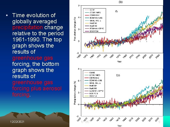
• Time evolution of globally averaged precipitation change relative to the period 1961 -1990. The top graph shows the results of greenhouse gas forcing, the bottom graph shows the results of greenhouse gas forcing plus aerosol forcing. 12/22/2021 UNBC 35

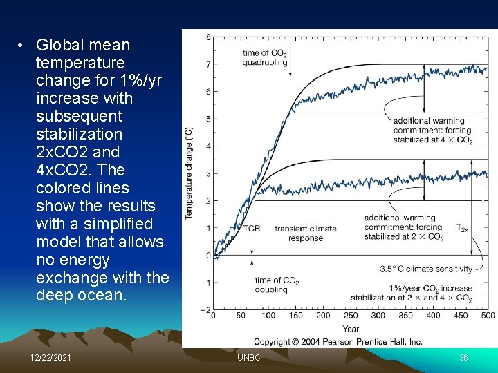
• Global mean temperature change for 1%/yr increase with subsequent stabilization 2 x. CO 2 and 4 x. CO 2. The colored lines show the results with a simplified model that allows no energy exchange with the deep ocean. 12/22/2021 UNBC 36

• Accuracy of models that predict global warming: (1) albedo errors (2) external factors not taken into consideration (3) model resolution (4) initial conditions (5) the role of clouds on climate changes 12/22/2021 UNBC 37

What limits success of climate models? • Processes occur on smaller scales that are different than those resolved on the larger scales. • These: a) affect the large scale rules b) change climate on scales that humans live on. • Have to some extent been recognized for long time – their inclusion has been called “parameterization” but better called “scaling”. 12/22/2021 UNBC 38

12/22/2021 UNBC 39

12/22/2021 UNBC 40

12/22/2021 UNBC 41

12/22/2021 UNBC 42

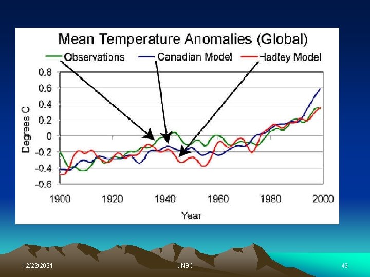
• Evidence of some uncertainties: (1) The individual models often exhibit worse agreement with observations. (2) All models have shortcomings in their simulations of the present day climate of the stratosphere, which might limit the accuracy of predictions of future climate change. (3) There are problems in simulating natural seasonal variability. (4) Coupled climate models do not simulate with reasonable accuracy clouds and some related hydrological processes. 12/22/2021 UNBC 43

• Evidence of model reliability: (1) The model mean exhibits good agreement with observations. (2) Surface air temperature is particularly well simulated. (3) For nearly all models the r. m. s. error in zonal- and annual-mean surface air temperature is small compared with its natural variability. 12/22/2021 UNBC 44

Conclusion ======= The majority of climatologists agree that important climate processes are imperfectly accounted for by the climate models but don't think that better models would change the conclusion. 12/22/2021 UNBC 45