Modeling Species Distribution with Max Ent Bryce Maxell

Modeling Species Distribution with Max. Ent Bryce Maxell, Acting Director, Montana Natural Heritage Program & Scott Story, Nongame Data Manager, Montana Fish, Wildlife and Parks

Agenda - Wednesday • • • 8 -9 9: 05 -10 10: 05 -11 11: 05 -12 12 -1 1 -1: 55 2 -3 3 -5 Tomorrow 8 -11 Introduction to Max. Ent Reptile and Amphibian Model Examples Installation and Walkthrough of Max. Ent Preparation of Data Lunch Thresholds & Model Validation Using models in your DSS Hands-on Session Hands-on, Data Prep, Questions & Discussion

• About to start again folks on the phone.

Installing and Running Max. Ent INSTALLATION

Download & Install • http: //www. cs. princeton. edu/~schapire/maxent/ • Current Max. Ent Version = 3. 3. 3 e • Requires Java Version 1. 4 or later • Type java –version at command prompt • http: //www. java. com • Extract the. zip file to a very simple directory – No spaces, no strange characters, short – C: maxent • Three files are installed – Maxent. bat – Maxent. jar – Readme. txt – Download the tutorial Word document

Check Java Version

Set PATH and customize. bat file • My Computer Properties Advanced Environment Variables System Variables PATH Edit • Add to end of the PATH ; c: maxent • Change the maxent. bat file – Change the extension to. txt so that you can edit it with Notepad 512 Mb = 0. 5 Gb 1024 = 1 Gb – Change line reading java -mx 512 m -jar maxent. jar 1536 = 1. 5 Gb to… 2048 = 2 Gb – java -mx 512 m -jar c: maxent. jar – Change the extension back to. bat – Note that changing the 512 to another number allocates more memory

Running Max. Ent BASIC MODELING RUN

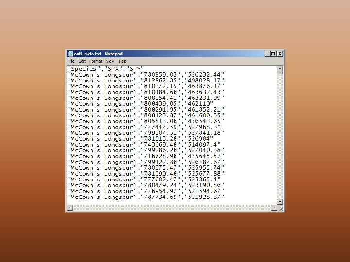
Required Inputs • Species presence localities (“samples”) file • Environmental feature layers • Output directory

Max. Ent – Main Screen

Supply presence localities

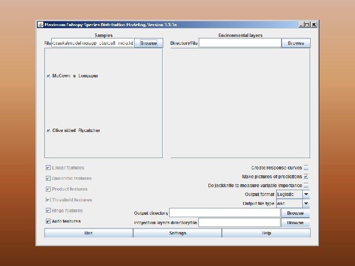
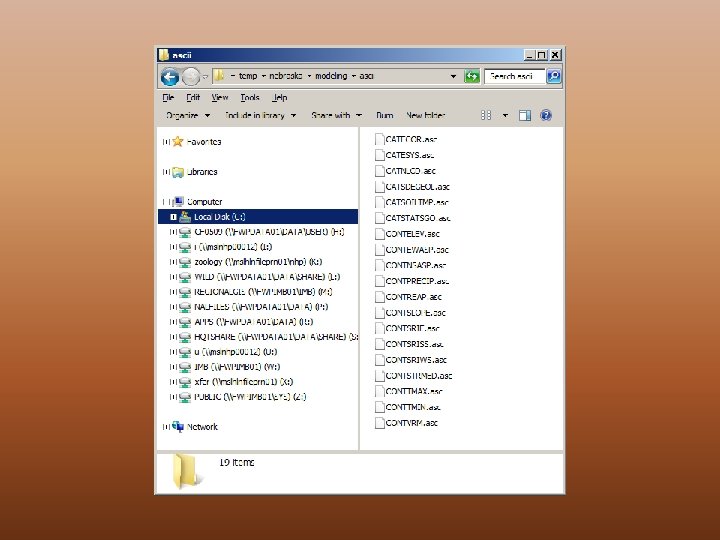
Supply folder containing environmental feature layers

Change variable types as necessary Supply an output directory

Ready to Run

What Max. Ent Does • Reads through each layer to – Determine type – Create. mxe file for each layer in maxent. cache • Extracts the random background and sample data – You will get warnings about points that are “missing some environmental data” • Calculates the gain until a threshold is reached • Creates the output grids for each species (this takes the longest) • Creates the thumbnail. png images

Time Required • Ten feature layers (3 categorical) – 46 million pixels • • • 2 Species Intel Core 2 Quad CPU (2. 83 GHz) 4. 00 GB RAM Without maxent. cache = 38 minutes With maxent. cache = 24 minutes Windows 7 32 -bit Operating System 512 Mb of memory specified

Running Max. Ent EXAMINING OUTPUT

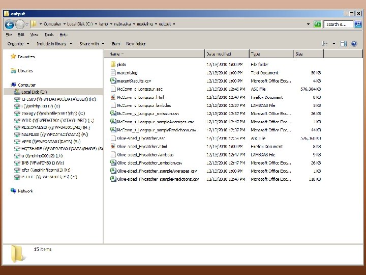
Output • • plots folder logfile maxent. Results. csv For each species –. asc –. html –. lambdas – _omission. csv – _sample. Averages. csv – _sample. Predictions. csv

• • • Logfile Timestamp Version of Max. Ent Samples file name Warnings Command line to repeat Species Layertypes Directories for: samples file, layers, output Number of samples Maximum gain

Gain • Closely related to deviance, a measure of GOF in GAM and GLM • Starts at zero and heads toward an asymptote • Max. Ent trying to come up with best fit • Average log probability of presence samples minus a constant • Gain indicates how closely the model is concentrated around presence samples • Avg likelihood of presence samples = exp(gain)

Gain Examples • Mc. Cown’s Longspur – Resulting gain: 2. 275 – Average likelihood for presence points = 9. 728 • Olive-sided Flycatcher – Resulting gain: 1. 297 – Average likelihood for presence points = 3. 658 • Average likelihood of the presence sample is X times higher than that of a background pixel

Html • • • Analysis of omission/commission Receiver Operating Curve (AUC calculated) Preset Thresholds Pictures of the Model Analysis of Variable Contributions Raw Outputs

Omission Rate vs. Cumulative Threshold

Receiver Operating Curve

Sample Predictions File • Coordinates for all points • Test or Training • Predicted values – Raw – Cumulative – Logistic • Use this file to calculate deviance • Use samples procedure in Arc. Map to extract the ones and zeros (above threshold or not)

Sample Predictions File

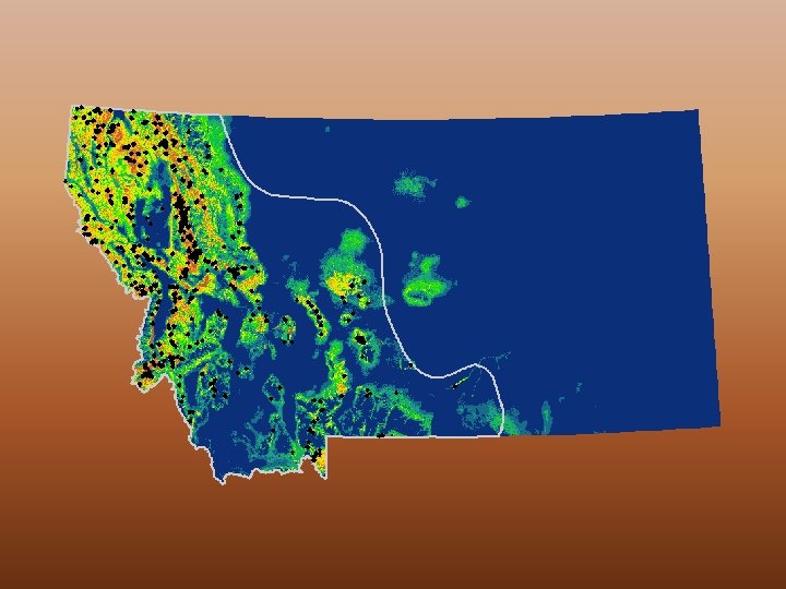
Logistic Ouput High probability of suitable conditions Low predicted probability of suitable conditions White dots = training (1059 points or 75%) Purple dots = test (352 points or 25%)

Viewing Data in Arc. Map • Build Raster Attribute Table (Categorical) –. vat. dbf • Build Histograms (Classified) –. aux • Build Pyramids –. rrd –. xml • For species output grids – Convert ASCII to Raster (Output Data Type = FLOATING) – Output as. bil (Band interleaved by line)

Running Max. Ent MORE ADVANCED PARAMETERS

Running Max. Ent REPLICATE RUNS

Running Max. Ent BATCH MODE

Preparation of Data Scott Story

Required Inputs • Species presence localities (“samples”) file • Environmental feature layers • Output directory

Getting Feature Data Ready • Same projection (coordinate system, units, datum) • Same resolution • Same extent • ESRI ascii format

Two Raster Datasets Land cover Precipitation • Source = Montana Natural Heritage Program • Type = IMAGINE Image • Cell size = 30 meters • Columns & Rows =33005, 24008 • Spatial Reference = Montana State Plane (NAD 83) • Pixel Type = Unsigned Integer (8 -bit) • Source = PRISM Climate Center • Type = ASCII grid • Cell size = 0. 0083333333 • Columns & Rows = 7025, 3105 • Spatial Reference = undefined (see metadata) • Pixel Type = Signed Integer (32 -bit)

Two Raster Datasets Land cover Precipitation

Making Rasters Match • Define coordinate systems for both • Set some environment variables – Tools Options Geoprocessing Tab Environments – General Settings: Extent and Snap Raster – Raster Analysis Settings: Cell Size, Mask • Project Raster – Select target raster to match for output cell size

Precipitation Reprojected & Resampled • Same exact extent • Same exact number or rows & columns • Same exact cell size • Real test is…does Maxent throw any errors? • In this case…it worked! • Getting all your data layers squared away will take some time!

Deriving New Raster Data Ruggedness

Types of Environmental Features • Continuous (Quantitative) – Interval-scale (interval data, order, linear scale) – Ordinal variables (scale unknown-transformed? , rank clear) – Ratio-scale (interval data, ordered, not on linear scale, e. g. temp on F or C scale) • Categorical (Qualitative) – Nominal (e. g. gender) – Ordinal (has order, e. g. low to great) – Dummy variables from quantitative (classes) • Name the ASCII files with CONT or CAT prefix

Preparing Point Data Create a separate file for each species Combine them allgroups of them into one file Probably want to retain a unique identifier May want to setup scripts in Arc. GIS to extract presence data • Might also want more control of how background data is selected • Let’s look at an example script Extract. Model. Input. Data. py • •

Other “Feature” Layers • Masks – useful if you want to train a model using only a subset of the region – mask. asc – containing a constant value (1, for example) in area of interest and no-data values everywhere else. • Bias – assumption that species occurrence data are unbiased – good understanding of the spatial pattern – values should indicate relative sampling effort

Representing the output THRESHOLDS

Logistic Output (Ranges 0 -1)

Reclassify with Arc. GIS

Preset Max. Ent Thresholds Cumulative Logistic Threshold Fractional Predicted Area Training Omission Rate Test Omission Rate Fixed Cumulative Value 1 1 0. 043 0. 344 0. 002 0. 000 Fixed Cumulative Value 5 5 0. 172 0. 255 0. 020 Fixed Cumulative Value 10 10 0. 260 0. 210 0. 044 0. 082 Minimum Training Presence 0. 699 0. 029 0. 365 0. 000 10 Percentile Training Presence 17. 522 0. 351 0. 167 0. 099 0. 151 Equal Training Sensitivity & Specificity 21. 989 0. 393 0. 149 0. 148 0. 205 Maximum Training Sensitivity Plus Specificity 9. 201 0. 248 0. 216 0. 035 0. 065 Equal test sensitivity & specificity 18. 603 0. 361 0. 162 0. 106 0. 162 Maximum test sensitivity plus specificity 7. 729 0. 225 0. 228 0. 029 0. 043 Balance Training Omission, 1. 054 Predicted Area, &Threshold Value 0. 047 0. 342 0. 000 Equate Entropy of Thresholded & Original Distributions 0. 182 0. 250 0. 021 0. 026 5. 465

Thresholds – Ends of Spectrum Balance Training Omission, Predicted Area, &Threshold Value Equal Training Sensitivity & Specificity

Model Validation MODEL VALIDATION

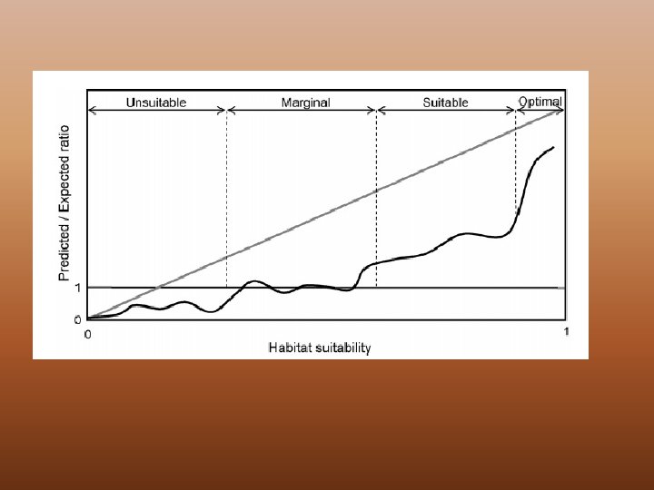
Validation Metrics • Receiver Operating Curve – obtained by plotting, for each threshold in this range, the proportion of true positive against the proportion of false positive • Area Under Curve – computed by computing the area under the above described curve • Deviance – 2 times the log probability of the test data. • Absolute Validation Index - the proportion of presence evaluation points falling above threshold or within the GAP predicted distribution • Point Biserial Correlation - The correlation between a model’s predictions and presence/absence in test data (regarded as a 01 variable)

_sample. Predictions. csv

Discussion Point

Topics Left • • • Data Prep Output Thresholds Validation Batch Replicates