Modeling Prediction Intervals using Monte Carlo Simulation Software

Modeling Prediction Intervals using Monte Carlo Simulation Software 2016 ICEAA Professional Development & Training Workshop James R. Black Qing Wu 17 Feb 2016 1

Presenter Bios • • James “Jay” Black has 12 years of cost estimating experience and currently works as senior operations research analyst for the Administration for Children and Families within the U. S. Department of Health and Human Services. In this role, he supports the Grants Center of Excellence software suite used to administer 1200 grant programs in eight Federal departments. Jay has a Masters in Systems Engineering from Johns Hopkins University and holds a current CCE/A certification. Qing “Q” Wu is a cost analyst for the Cost Effectiveness Branch at the Naval Surface Warfare Center Carderock Division. She supports the Naval Sea Systems Command 05 C Cost Engineering & Industrial Analysis Division in their Weapon Systems Division. She has a Bachelor’s degree in Mathematics from the Macaulay Honors College at The City College of New York. 2

Presentation Summary • References/Acknowledgements: – 2014 ICEAA Workshop presentation prepared by Dr. Christian Smart (MDA) and Marc Greenberg (NASA) – Joint Agency Cost Schedule Risk and Uncertainty Handbook (CSRUH, Feb 2014) • Abstract: – The use of a prediction interval (PI) is a simple method of quantifying risk and uncertainty for a Cost Estimating Relationship (CER) derived from an Ordinary Least Squares (OLS) regression – Yet, few cost estimators implement PIs in their estimates despite their frequent use of CERs This presentation will provide a step-by-step tutorial for modeling a PI for an example CER using Monte Carlo Simulation software and will identify the beneficial impact on the coefficient of variation (CV) 3

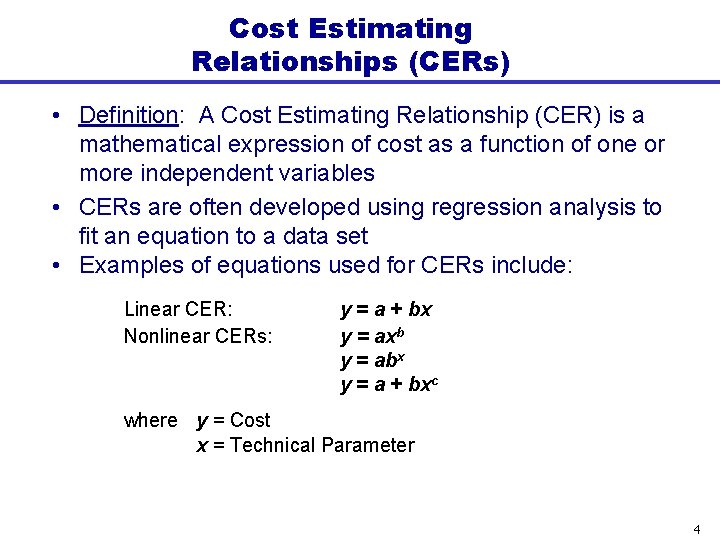
Cost Estimating Relationships (CERs) • Definition: A Cost Estimating Relationship (CER) is a mathematical expression of cost as a function of one or more independent variables • CERs are often developed using regression analysis to fit an equation to a data set • Examples of equations used for CERs include: Linear CER: Nonlinear CERs: y = a + bx y = axb y = abx y = a + bxc where y = Cost x = Technical Parameter 4

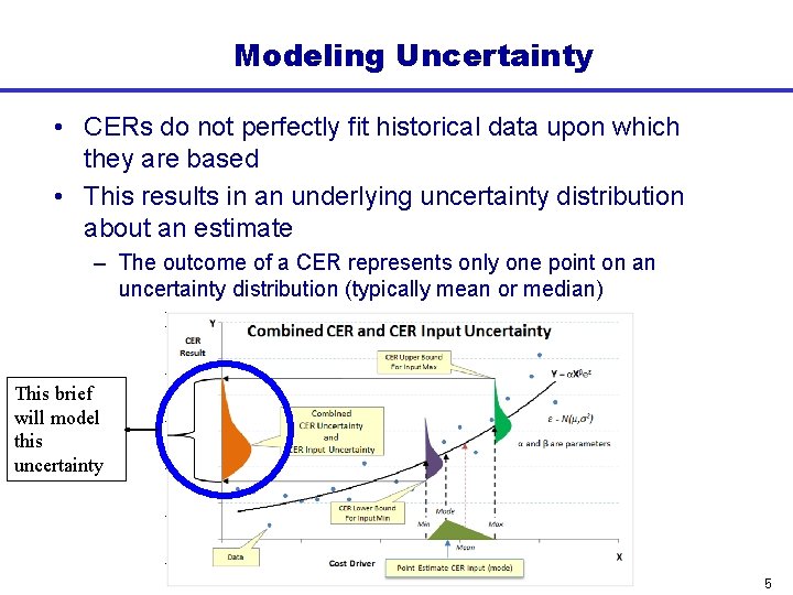
Modeling Uncertainty • CERs do not perfectly fit historical data upon which they are based • This results in an underlying uncertainty distribution about an estimate – The outcome of a CER represents only one point on an uncertainty distribution (typically mean or median) This brief will model this uncertainty 5

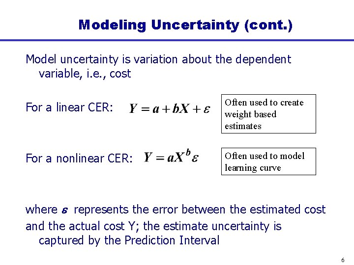
Modeling Uncertainty (cont. ) Model uncertainty is variation about the dependent variable, i. e. , cost For a linear CER: Often used to create weight based estimates For a nonlinear CER: Often used to model learning curve where e represents the error between the estimated cost and the actual cost Y; the estimate uncertainty is captured by the Prediction Interval 6

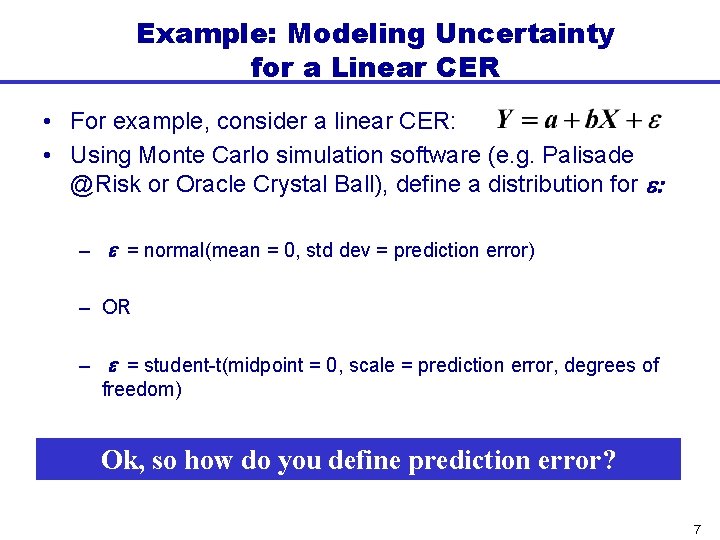
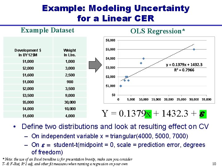
Example: Modeling Uncertainty for a Linear CER • For example, consider a linear CER: • Using Monte Carlo simulation software (e. g. Palisade @Risk or Oracle Crystal Ball), define a distribution for e: – e = normal(mean = 0, std dev = prediction error) – OR – e = student-t(midpoint = 0, scale = prediction error, degrees of freedom) Ok, so how do you define prediction error? 7

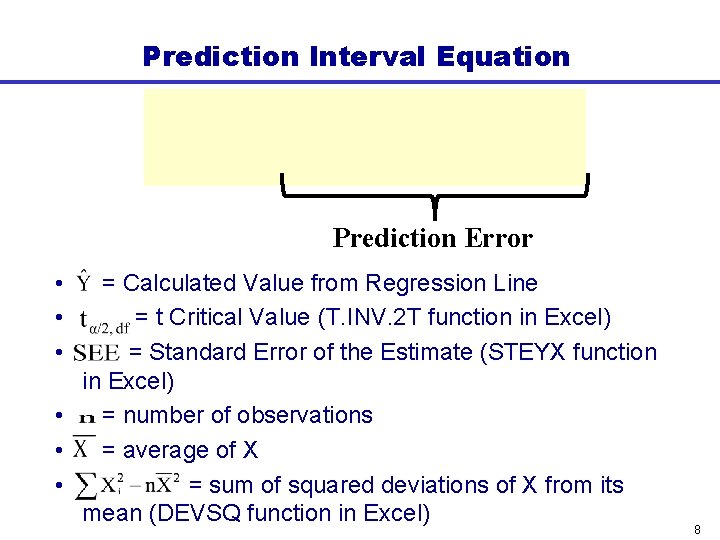
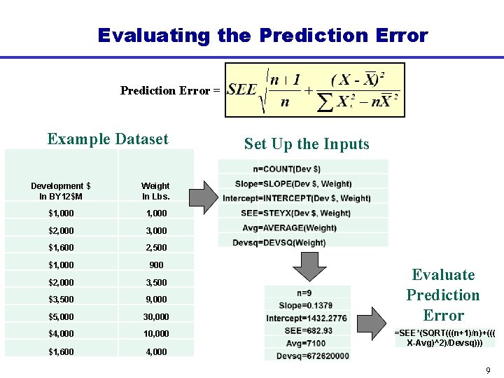
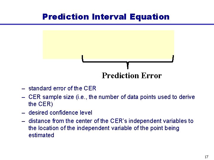
Prediction Interval Equation Prediction Error • • • = Calculated Value from Regression Line = t Critical Value (T. INV. 2 T function in Excel) = Standard Error of the Estimate (STEYX function in Excel) • = number of observations • = average of X • = sum of squared deviations of X from its mean (DEVSQ function in Excel) 8

Evaluating the Prediction Error = Example Dataset Development $ In BY 12$M Weight In Lbs. $1, 000 $2, 000 3, 000 $1, 600 2, 500 $1, 000 900 $2, 000 3, 500 $3, 500 9, 000 $5, 000 30, 000 $4, 000 10, 000 $1, 600 4, 000 Set Up the Inputs Evaluate Prediction Error =SEE*(SQRT(((n+1)/n)+((( X-Avg)^2)/Devsq))) 9

Example: Modeling Uncertainty for a Linear CER Example Dataset Development $ In BY 12$M Weight In Lbs. $1, 000 $2, 000 3, 000 $1, 600 2, 500 $1, 000 900 $2, 000 3, 500 $3, 500 9, 000 $5, 000 30, 000 $4, 000 10, 000 $1, 600 4, 000 OLS Regression* Y = 0. 1379 x + 1432. 3 + e • Define two distributions and look at resulting effect on CV – On independent variable x = triangular(4000, 5000, 7000) – On e = student-t(midpoint = 0, scale = prediction error, degrees of freedom) * Note: the use of an Excel trendline is for presentation brevity, make sure you consider T- & F-Stat, R^2 adj, and other fit measures when running a regression on your own 10

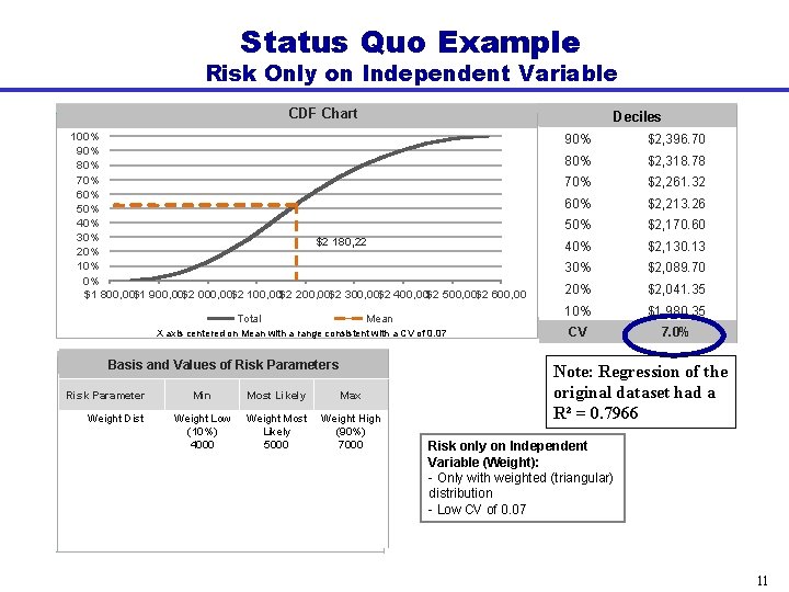
Status Quo Example Risk Only on Independent Variable CDF Chart Deciles 100% 90% 80% 70% 60% 50% 40% 30% $2 180, 22 20% 10% 0% $1 800, 00$1 900, 00$2 000, 00$2 100, 00$2 200, 00$2 300, 00$2 400, 00$2 500, 00$2 600, 00 Total Mean X axis centered on Mean with a range consistent with a CV of 0. 07 Basis and Values of Risk Parameters Risk Parameter Weight Dist Min Most Likely Max Weight Low (10%) 4000 Weight Most Likely 5000 Weight High (90%) 7000 90% $2, 396. 70 80% $2, 318. 78 70% $2, 261. 32 60% $2, 213. 26 50% $2, 170. 60 40% $2, 130. 13 30% $2, 089. 70 20% $2, 041. 35 10% CV CV $1, 980. 35 5. 2% 7. 0% Note: Regression of the original dataset had a R² = 0. 7966 Risk only on Independent Variable (Weight): - Only with weighted (triangular) distribution - Low CV of 0. 07 11

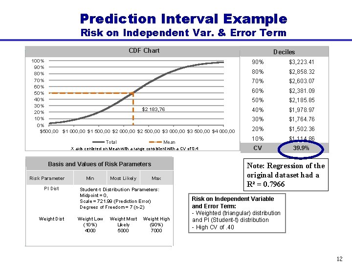
Prediction Interval Example Risk on Independent Var. & Error Term CDF Chart Deciles 100% 90% 80% 70% 60% 50% 40% 30% $2 183, 76 20% 10% 0% $500, 00 $1 000, 00 $1 500, 00 $2 000, 00 $2 500, 00 $3 000, 00 $3 500, 00 $4 000, 00 Total Mean X axis centered on Mean with a range consistent with a CV of 0. 4 Basis and Values of Risk Parameters Risk Parameter PI Dist Weight Dist Min Most Likely Max Student-t Distribution Parameters: Midpoint = 0, Scale = 721. 99 (Prediction Error) Degrees of Freedom = 7 (n-2) Weight Low (10%) 4000 Weight Most Likely 5000 Weight High (90%) 7000 90% $3, 223. 41 80% $2, 858. 32 70% $2, 603. 07 60% $2, 381. 09 50% $2, 185. 85 40% $1, 978. 97 30% $1, 764. 76 20% $1, 502. 36 10% CV CV $1, 114. 86 5. 2% 39. 9% Note: Regression of the original dataset had a R² = 0. 7966 Risk on Independent Variable and Error Term: - Weighted (triangular) distribution and PI (Student-t) distribution - High CV of. 40 12

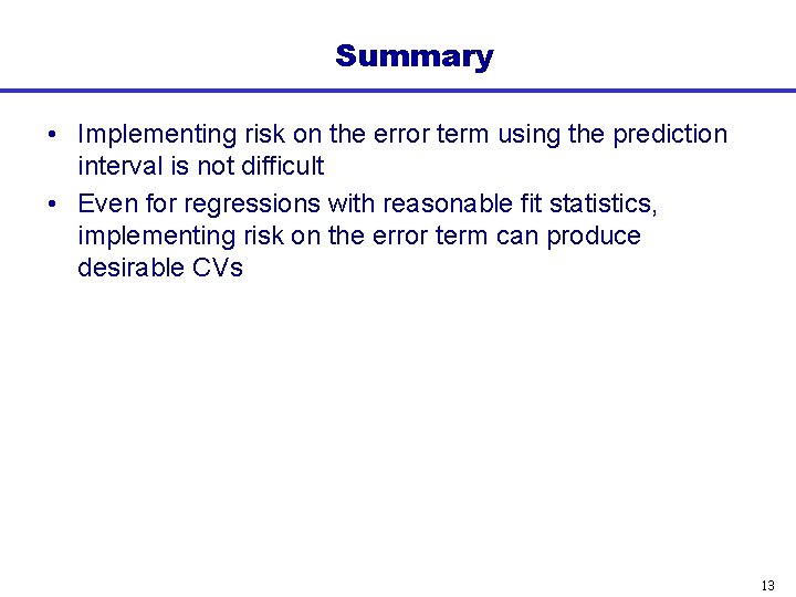
Summary • Implementing risk on the error term using the prediction interval is not difficult • Even for regressions with reasonable fit statistics, implementing risk on the error term can produce desirable CVs 13

BACKUP 14

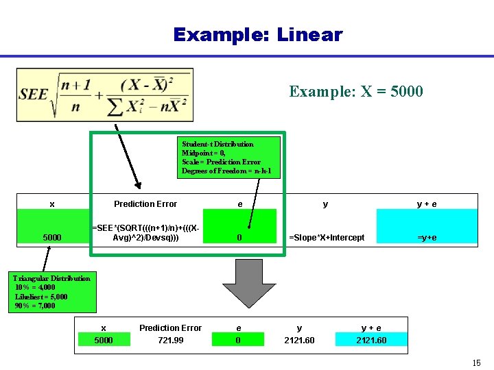
Example: Linear Example: X = 5000 Student-t Distribution Midpoint = 0, Scale = Prediction Error Degrees of Freedom = n-k-1 x Prediction Error e y y+e 5000 =SEE*(SQRT(((n+1)/n)+(((XAvg)^2)/Devsq))) 0 =Slope*X+Intercept =y+e Triangular Distribution 10% = 4, 000 Likeliest = 5, 000 90% = 7, 000 x Prediction Error e y y+e 5000 721. 99 0 2121. 60 15

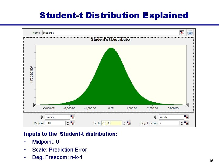
Student-t Distribution Explained Inputs to the Student-t distribution: • Midpoint: 0 • Scale: Prediction Error • Deg. Freedom: n-k-1 16

Prediction Interval Equation Prediction Error – standard error of the CER – CER sample size (i. e. , the number of data points used to derive the CER) – desired confidence level – distance from the center of the CER’s independent variables to the location of the independent variable of the point being estimated 17

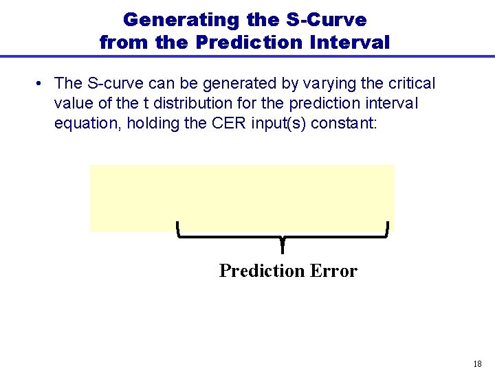
Generating the S-Curve from the Prediction Interval • The S-curve can be generated by varying the critical value of the t distribution for the prediction interval equation, holding the CER input(s) constant: Prediction Error 18

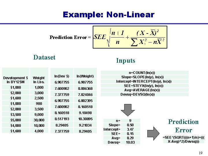
Example: Non-Linear Prediction Error = Dataset Inputs Development $ In BY 12$M Weight In Lbs. ln(Dev $) ln(Weight) 6. 907755 $1, 000 7. 600902 8. 006368 $2, 000 3, 000 $1, 600 2, 500 7. 377759 7. 824046 $1, 000 900 6. 907755 6. 802395 $2, 000 3, 500 7. 600902 8. 160518 $3, 500 9, 000 8. 160518 9. 10498 $5, 000 30, 000 8. 517193 10. 30895 $4, 000 10, 000 8. 29405 9. 21034 $1, 600 4, 000 7. 377759 8. 29405 n=COUNT(ln(x)) Slope=SLOPE(ln(y), ln(x)) Intercept=INTERCEPT(ln(y), ln(x)) SEE=STEYX(ln(y), ln(x)) Avg=AVERAGE(ln(x)) Devsq=DEVSQ(ln(x)) n= Slope= Intercept= SEE= Avg= Devsq= 9 0. 50 3. 47 0. 15 8. 29 10. 03 Prediction Error =SEE*(SQRT(((n+1)/n)+((( X-Avg)^2)/Devsq))) 19

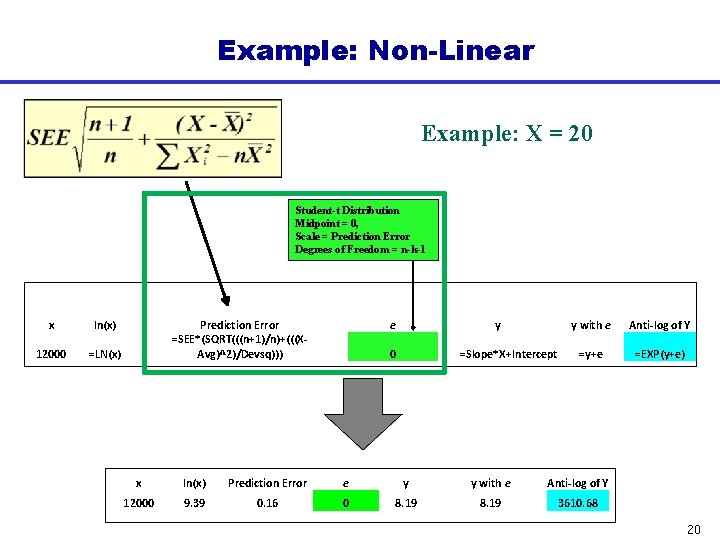
Example: Non-Linear Example: X = 20 Student-t Distribution Midpoint = 0, Scale = Prediction Error Degrees of Freedom = n-k-1 x ln(x) 12000 =LN(x) Prediction Error =SEE*(SQRT(((n+1)/n)+(((XAvg)^2)/Devsq))) e y 0 =Slope*X+Intercept y with e Anti-log of Y =y+e =EXP(y+e) x ln(x) Prediction Error e y y with e Anti-log of Y 12000 9. 39 0. 16 0 8. 19 3610. 68 20

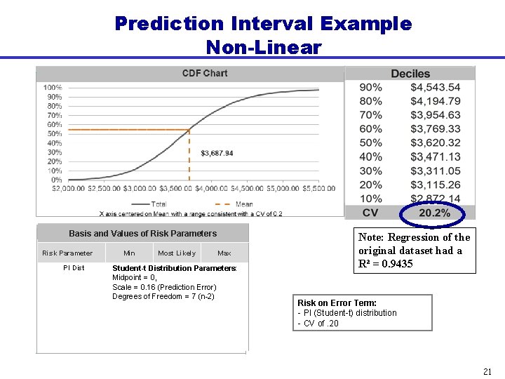
Prediction Interval Example Non-Linear Deciles CV Basis and Values of Risk Parameters Risk Parameter PI Dist Min Most Likely Max Student-t Distribution Parameters: Midpoint = 0, Scale = 0. 16 (Prediction Error) Degrees of Freedom = 7 (n-2) 5. 2% Note: Regression of the original dataset had a R² = 0. 9435 Risk on Error Term: - PI (Student-t) distribution - CV of. 20 21

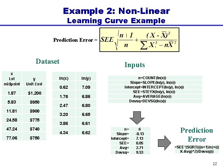
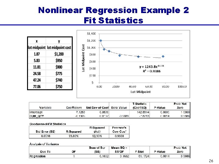
Example 2: Non-Linear Learning Curve Example Prediction Error = Dataset x Lot midpoint y Unit Cost 1. 87 $1, 200 5. 83 $950 11. 81 $900 24. 58 $775 47. 24 $740 77. 06 $750 Inputs ln(x) ln(y) 0. 62 7. 09 1. 76 6. 86 2. 47 6. 80 3. 20 6. 65 3. 86 6. 61 4. 34 6. 62 n=COUNT(ln(x)) Slope=SLOPE(ln(y), ln(x)) Intercept=INTERCEPT(ln(y), ln(x)) SEE=STEYX(ln(y), ln(x)) Avg=AVERAGE(ln(x)) Devsq=DEVSQ(ln(x)) n= Slope= Intercept= SEE= Avg= Devsq= 6 -0. 13 7. 13 0. 05 2. 71 9. 53 Prediction Error =SEE*(SQRT(((n+1)/n)+((( X-Avg)^2)/Devsq))) 22

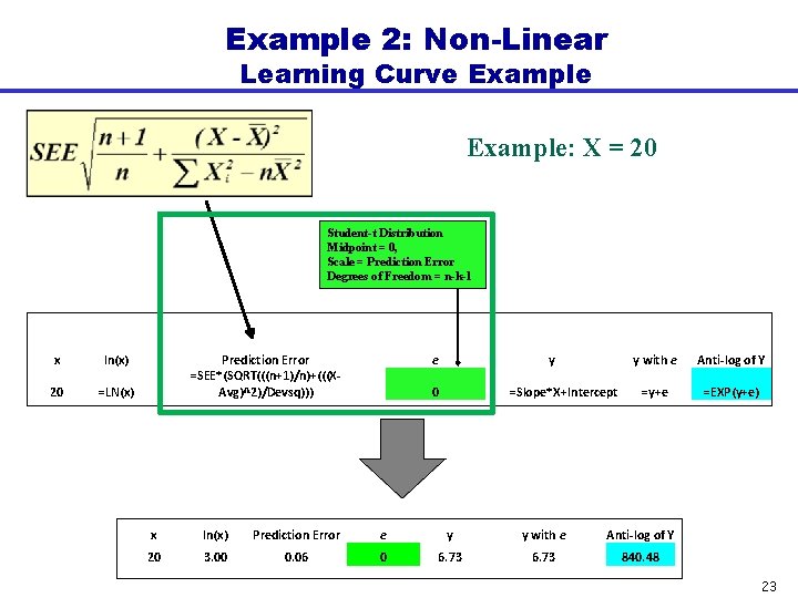
Example 2: Non-Linear Learning Curve Example: X = 20 Student-t Distribution Midpoint = 0, Scale = Prediction Error Degrees of Freedom = n-k-1 x ln(x) 20 =LN(x) Prediction Error =SEE*(SQRT(((n+1)/n)+(((XAvg)^2)/Devsq))) e y 0 =Slope*X+Intercept y with e Anti-log of Y =y+e =EXP(y+e) x ln(x) Prediction Error e y y with e Anti-log of Y 20 3. 00 0. 06 0 6. 73 840. 48 23

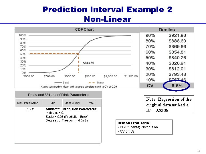
Prediction Interval Example 2 Non-Linear Deciles CV Basis and Values of Risk Parameters Risk Parameter PI Dist Min Most Likely Max Student-t Distribution Parameters: Midpoint = 0, Scale = 0. 06 (Prediction Error) Degrees of Freedom = 4 (n-2) 5. 2% Note: Regression of the original dataset had a R² = 0. 9386 Risk on Error Term: - PI (Student-t) distribution - CV of. 09 24

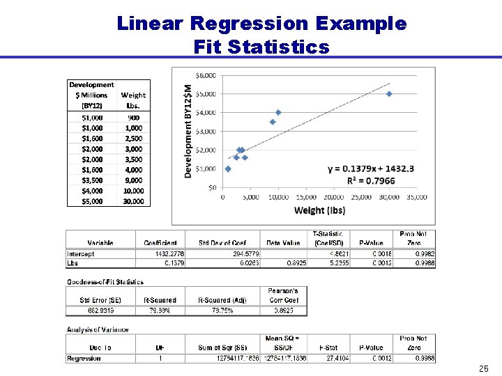
Linear Regression Example Fit Statistics 25

Nonlinear Regression Example 2 Fit Statistics 26