Modeling Flows and Information Single commodity flow problems

Modeling Flows and Information Single commodity flow problems Multicommodity Flow Conservation Weight and Cube Pass through vs Unload/Reload Tracking Information Column Generation 1 15. 057 Spring 02 Vande Vate 1

Modeling Tools • We will rely on Solver in Excel • Instructions on installing and using Solver accessible from the class homepage • Convenient: – Everyone is familiar with Excel – Minimal fixed costs of installing, accessing and learning syntax for a new application • Inconvenient: – – – Solver is unreliable. It says models are not linear when they are. It says it has found a solution when it hasn't, etc. It combines the problem data with the model 2 15. 057 Spring 02 Vande Vate 2 Limited problem sizes

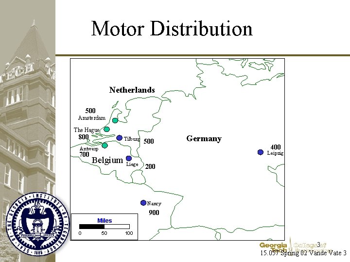
Motor Distribution Netherlands 500 Amsterdam The Hague * 800 * Antwerp 700 * * Belgium 500 800 Tilburg 500 700 * Liege 200 * 200 Germany 400 * Leipzig 400 Nancy 900 Miles 0 50 100 3 15. 057 Spring 02 Vande Vate 3

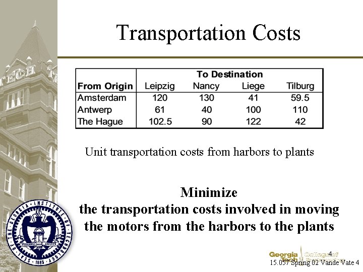
Transportation Costs Unit transportation costs from harbors to plants Minimize the transportation costs involved in moving the motors from the harbors to the plants 4 15. 057 Spring 02 Vande Vate 4

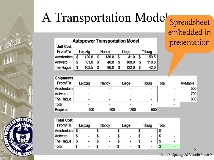
A Transportation Model Spreadsheet embedded in presentation 5 15. 057 Spring 02 Vande Vate 5

Challenge • Find a best answer 6 15. 057 Spring 02 Vande Vate 6

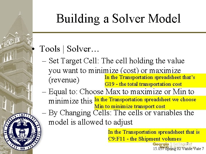
Building a Solver Model • Tools | Solver… – Set Target Cell: The cell holding the value you want to minimize (cost) or maximize In the Transportation spreadsheet that’s (revenue) G 19 - the total transportation cost – Equal to: Choose Max to maximize or Min to minimize this In the Transportation spreadsheet we choose Min to minimize transport cost – By Changing Cells: The cells or variables the model is allowed to adjust In the Transportation spreadsheet that is C 9: F 11 - the Shipment volumes 7 15. 057 Spring 02 Vande Vate 7

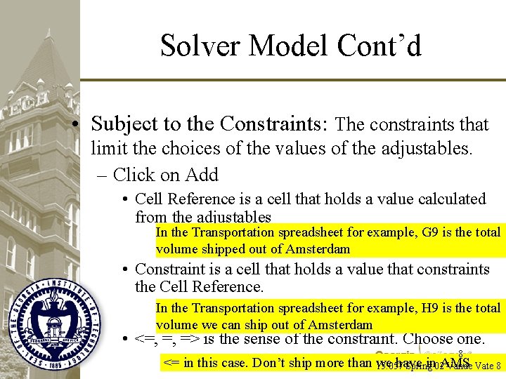
Solver Model Cont’d • Subject to the Constraints: The constraints that limit the choices of the values of the adjustables. – Click on Add • Cell Reference is a cell that holds a value calculated from the adjustables In the Transportation spreadsheet for example, G 9 is the total volume shipped out of Amsterdam • Constraint is a cell that holds a value that constraints the Cell Reference. In the Transportation spreadsheet for example, H 9 is the total volume we can ship out of Amsterdam • <=, =, => is the sense of the constraint. Choose one. 8 <= in this case. Don’t ship more than we have in 02 AMS 15. 057 Spring Vande Vate 8

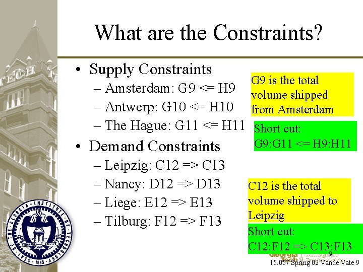
What are the Constraints? • Supply Constraints G 9 is the total volume shipped from Amsterdam – Amsterdam: G 9 <= H 9 – Antwerp: G 10 <= H 10 – The Hague: G 11 <= H 11 Short cut: • Demand Constraints – Leipzig: C 12 => C 13 – Nancy: D 12 => D 13 – Liege: E 12 => E 13 – Tilburg: F 12 => F 13 G 9: G 11 <= H 9: H 11 C 12 is the total volume shipped to Leipzig Short cut: C 12: F 12 => C 13: F 13 9 15. 057 Spring 02 Vande Vate 9

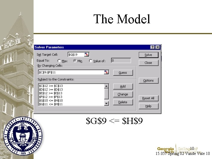
The Model $G$9 <= $H$9 10 15. 057 Spring 02 Vande Vate 10

What’s Missing? 11 15. 057 Spring 02 Vande Vate 11

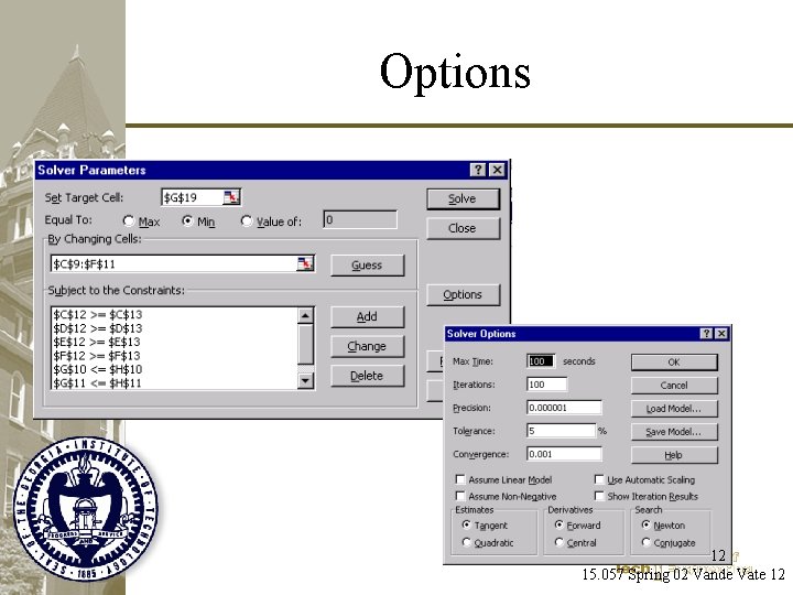
Options 12 15. 057 Spring 02 Vande Vate 12

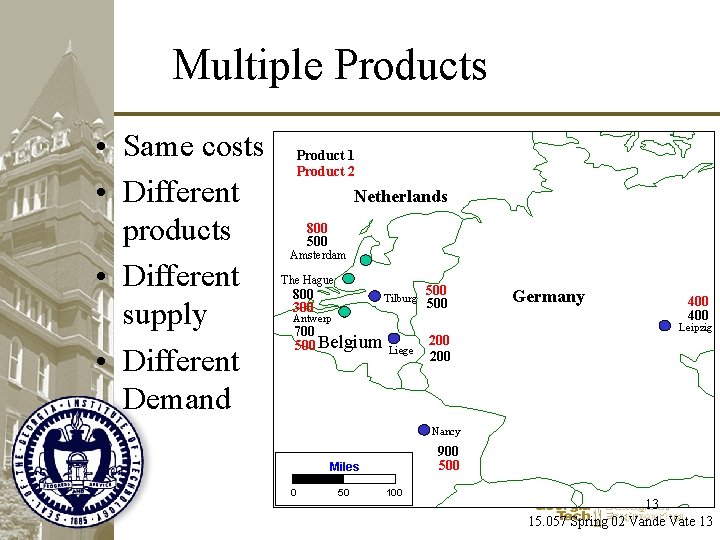
Multiple Products • Same costs • Different products • Different supply • Different Demand Product 1 Product 2 Netherlands 800 500 Amsterdam The Hague 800 300 * * * Antwerp * 700 500 Belgium 500 800 500 Tilburg 500 700 * Liege 200 * 50 400 * Leipzig 400 Nancy 900 500 Miles 0 200 Germany 100 13 15. 057 Spring 02 Vande Vate 13

Question • Can we just combine the products: – Total Supply at each source – Total Demand at each destination • The Hague – Total Supply: 1, 100 = 800 + 300 • Tilburg – Total Demand: 1, 000 = 500 + 500 14 15. 057 Spring 02 Vande Vate 14

Question • Can we just solve two separate problems: – One Problem for Product 1 – One Problem for Product 2? 15 15. 057 Spring 02 Vande Vate 15

Question • Can we just solve two separate problems: – One Problem for Product 1 – One Problem for Product 2? • When won’t this work? – Different Costs? – Capacities on Transportation –. . . 16 15. 057 Spring 02 Vande Vate 16

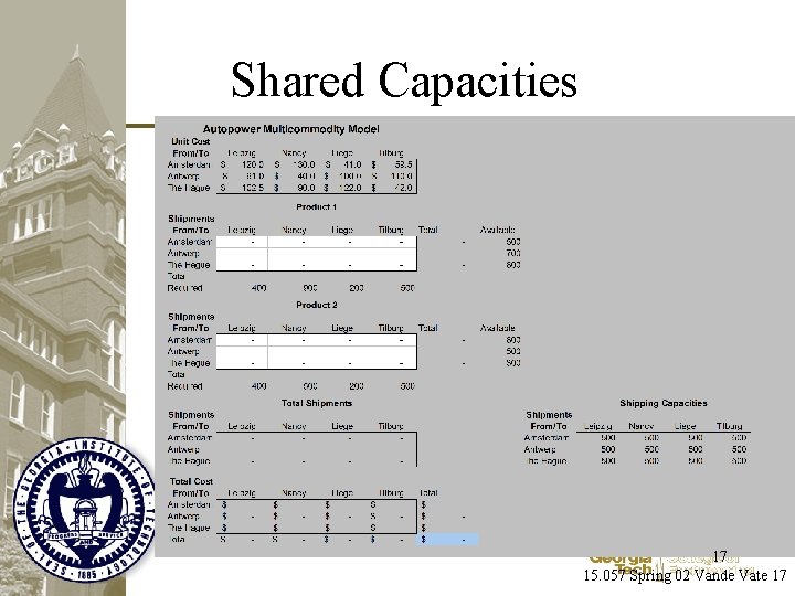
Shared Capacities 17 15. 057 Spring 02 Vande Vate 17

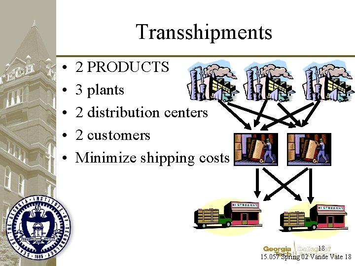
Transshipments • • • 2 PRODUCTS 3 plants 2 distribution centers 2 customers Minimize shipping costs 18 15. 057 Spring 02 Vande Vate 18

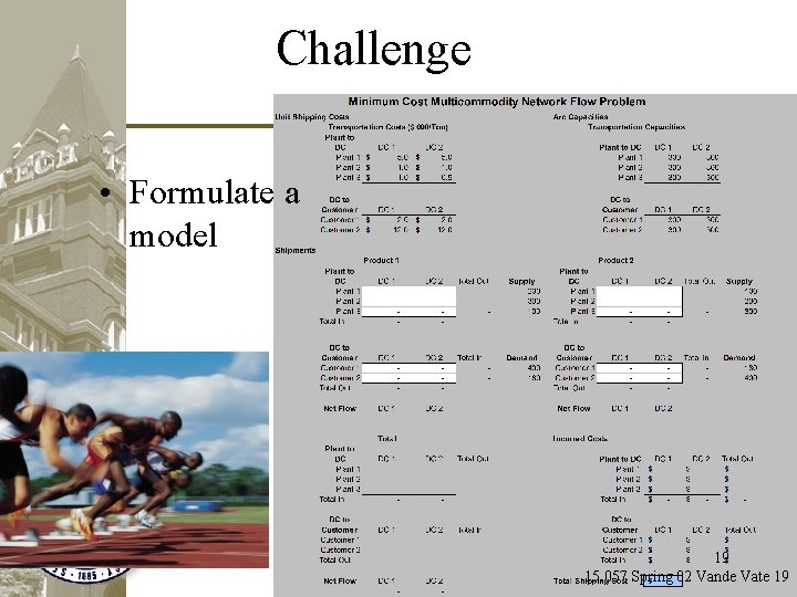
Challenge • Formulate a model 19 15. 057 Spring 02 Vande Vate 19

Flow Conservation • Conserve Flow at the DC – Product by Product • Otherwise… – Alchemy: Turn lead into gold 20 15. 057 Spring 02 Vande Vate 20

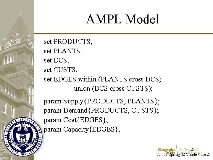
AMPL Model set PRODUCTS; set PLANTS; set DCS; set CUSTS; set EDGES within (PLANTS cross DCS) union (DCS cross CUSTS); param Supply{PRODUCTS, PLANTS}; param Demand{PRODUCTS, CUSTS}; param Cost{EDGES}; param Capacity{EDGES}; 21 15. 057 Spring 02 Vande Vate 21

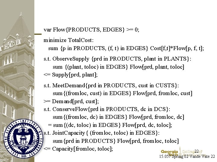
var Flow{PRODUCTS, EDGES} >= 0; minimize Total. Cost: sum {p in PRODUCTS, (f, t) in EDGES} Cost[f, t]*Flow[p, f, t]; s. t. Observe. Supply {prd in PRODUCTS, plant in PLANTS}: sum {(plant, toloc) in EDGES} Flow[prd, plant, toloc] <= Supply[prd, plant]; s. t. Meet. Demand{prd in PRODUCTS, cust in CUSTS}: sum{(fromloc, cust) in EDGES} Flow[prd, fromloc, cust] >= Demand[prd, cust]; s. t. Conserve. Flow{prd in PRODUCTS, dc in DCS}: sum{(fromloc, dc) in EDGES} Flow[prd, fromloc, dc] = sum{(dc, toloc) in EDGES} Flow[prd, dc, toloc]; s. t. Joint. Capacity{ (fromloc, toloc) in EDGES}: sum{prd in PRODUCTS} Flow[prd, fromloc, toloc] <= Capacity[fromloc, toloc]; 22 15. 057 Spring 02 Vande Vate 22

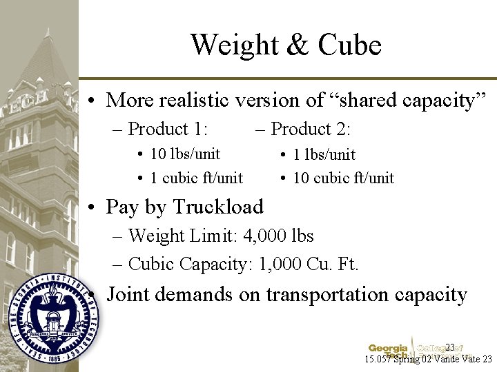
Weight & Cube • More realistic version of “shared capacity” – Product 1: – Product 2: • 10 lbs/unit • 1 cubic ft/unit • 1 lbs/unit • 10 cubic ft/unit • Pay by Truckload – Weight Limit: 4, 000 lbs – Cubic Capacity: 1, 000 Cu. Ft. • Joint demands on transportation capacity 23 15. 057 Spring 02 Vande Vate 23

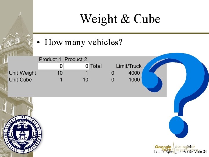
Weight & Cube • How many vehicles? 24 15. 057 Spring 02 Vande Vate 24

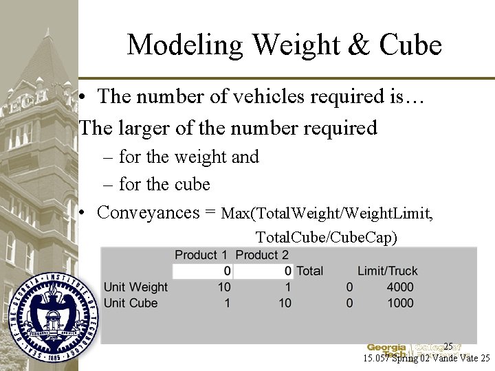
Modeling Weight & Cube • The number of vehicles required is… The larger of the number required – for the weight and – for the cube • Conveyances = Max(Total. Weight/Weight. Limit, Total. Cube/Cube. Cap) 25 15. 057 Spring 02 Vande Vate 25

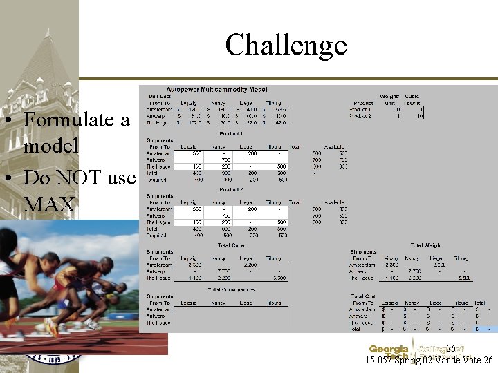
Challenge • Formulate a model • Do NOT use MAX 26 15. 057 Spring 02 Vande Vate 26

More Detail • Container at a port • Container at a distribution center • Container at a port – Conserve flow of containers – Goods in the containers don’t change • Container at a distribution center – Conserve flow of goods – Loads change from in-bound to outbound 27 15. 057 Spring 02 Vande Vate 27

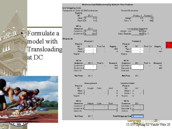
Challenge • Formulate a model with Transloading at DC 28 15. 057 Spring 02 Vande Vate 28

Without Transloading • • Same number of conveyances in and out Same products in those conveyances Lose potential to improve capacity utilization How to model? 29 15. 057 Spring 02 Vande Vate 29

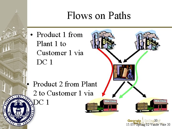
Flows on Paths • Product 1 from Plant 1 to Customer 1 via DC 1 • Product 2 from Plant 2 to Customer 1 via DC 1 30 15. 057 Spring 02 Vande Vate 30

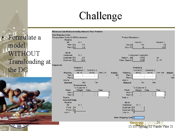
Challenge • Formulate a model WITHOUT Transloading at the DC 31 15. 057 Spring 02 Vande Vate 31

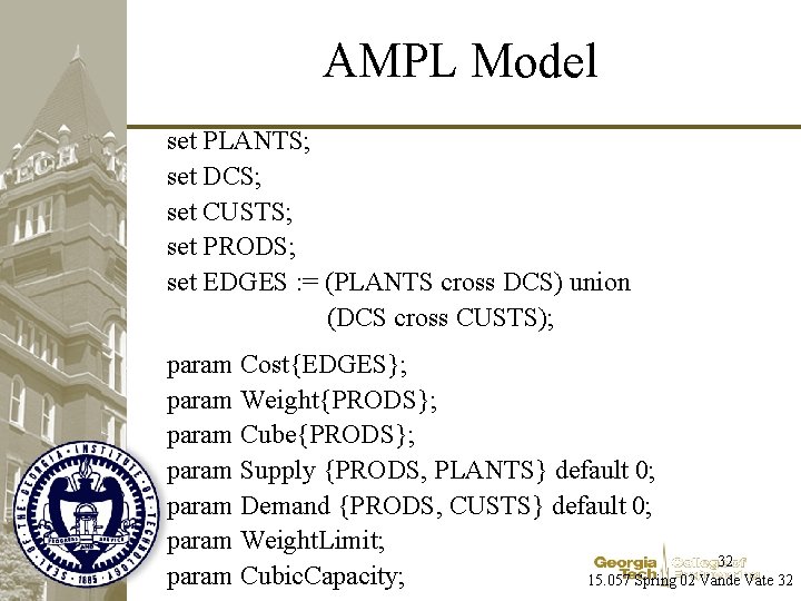
AMPL Model set PLANTS; set DCS; set CUSTS; set PRODS; set EDGES : = (PLANTS cross DCS) union (DCS cross CUSTS); param Cost{EDGES}; param Weight{PRODS}; param Cube{PRODS}; param Supply {PRODS, PLANTS} default 0; param Demand {PRODS, CUSTS} default 0; param Weight. Limit; 32 param Cubic. Capacity; 15. 057 Spring 02 Vande Vate 32

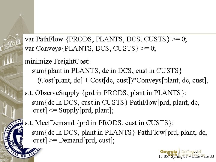
var Path. Flow {PRODS, PLANTS, DCS, CUSTS} >= 0; var Conveys{PLANTS, DCS, CUSTS} >= 0; minimize Freight. Cost: sum{plant in PLANTS, dc in DCS, cust in CUSTS} (Cost[plant, dc] + Cost[dc, cust])*Conveys[plant, dc, cust]; s. t. Observe. Supply {prd in PRODS, plant in PLANTS}: sum{dc in DCS, cust in CUSTS} Path. Flow[prd, plant, dc, cust] <= Supply[prd, plant]; s. t. Meet. Demand {prd in PRODS, cust in CUSTS}: sum{dc in DCS, plant in PLANTS} Path. Flow[prd, plant, dc, cust] >= Demand[prd, cust]; 33 15. 057 Spring 02 Vande Vate 33

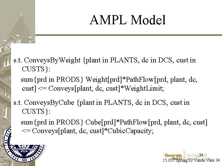
AMPL Model s. t. Conveys. By. Weight {plant in PLANTS, dc in DCS, cust in CUSTS}: sum{prd in PRODS} Weight[prd]*Path. Flow[prd, plant, dc, cust] <= Conveys[plant, dc, cust]*Weight. Limit; s. t. Conveys. By. Cube {plant in PLANTS, dc in DCS, cust in CUSTS}: sum{prd in PRODS} Cube[prd]*Path. Flow[prd, plant, dc, cust] <= Conveys[plant, dc, cust]*Cubic. Capacity; 34 15. 057 Spring 02 Vande Vate 34

Other Uses • Additional Information about the products history – Where it was made for • • Duties Pipeline Inventory How long it has been traveling … • Extreme cases: very long involved paths 35 15. 057 Spring 02 Vande Vate 35

Column Generation • Airlines Crew Scheduling – Complex pay and duty rules • Unions • FAA – Tour of duty for a crew • Several legs returning to base • Millions of possible tours of duty • Each is a variable: – 1 = use it in schedule – 0 = do not. 36 15. 057 Spring 02 Vande Vate 36

Solution Strategy • Initial Tours of Duty – Used in previous solutions – Fillers to ensure feasibility • Repeat until Done – Solve small problem – Use Shadow Prices to generate new tours that will improve solution – When no better tours are found -- done 37 15. 057 Spring 02 Vande Vate 37

Column Generation Example • Multicommodity Flow 38 15. 057 Spring 02 Vande Vate 38

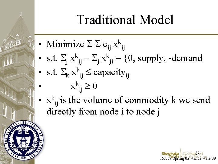
Traditional Model • • • Minimize S S cij xkij s. t. Sj xkij – Sj xkji = {0, supply, -demand s. t. Sk xkij capacityij xkij 0 xkij is the volume of commodity k we send directly from node i to node j 39 15. 057 Spring 02 Vande Vate 39

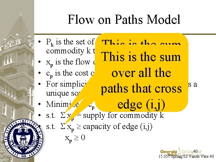
Flow on Paths Model • Pk is the set of paths from the source for This is the sum commodity k to the destination. is the sum • xp is the flow on. This path p over all the • cp is the cost of oneover unit of flow on path p all the paths for • For simplicity assume each commodity has a paths that cross unique source and a unique destination commodity k • Minimize S cp xp edge (i, j) • s. t. S xp = supply for commodity k • s. t. S xp capacity of edge (i, j) • xp 0 40 15. 057 Spring 02 Vande Vate 40

Flows On Paths Formulation • Variable for – Product 1: Each path from 1 to 5 – Product 2: Each path from 2 to 4 • Constraints: Capacity on each edge: – Sum of flows on paths that use the edge do not exceed capacity of the edge • Cost: Each unit of flow on a path pays the cost of all the edges on the path • Why no Flow Conservation Constraints? 41 15. 057 Spring 02 Vande Vate 41

Column Generation Approach • Start with 2 paths – Product 1: The edge from 1 to 5 – Product 2: The edge from 2 to 4 • Solve and get Shadow Prices on the capacity constraints • Calculate new (shortest) paths with the best reduced costs • Repeat. 42 15. 057 Spring 02 Vande Vate 42

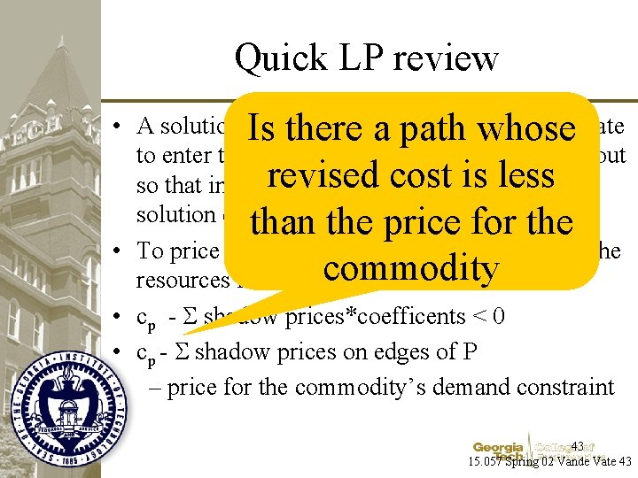
Quick LP review • A solution is variablewhose is a candidate Isoptimal thereif ano path to enter the basis. That is if no variable prices out revised costdecreases is lessthe so that increasing the variable solution cost. than the price for the • To price out a variable, compare its cost with the commodity resources it consumes • cp - S shadow prices*coefficents < 0 • cp - S shadow prices on edges of P – price for the commodity’s demand constraint 43 15. 057 Spring 02 Vande Vate 43

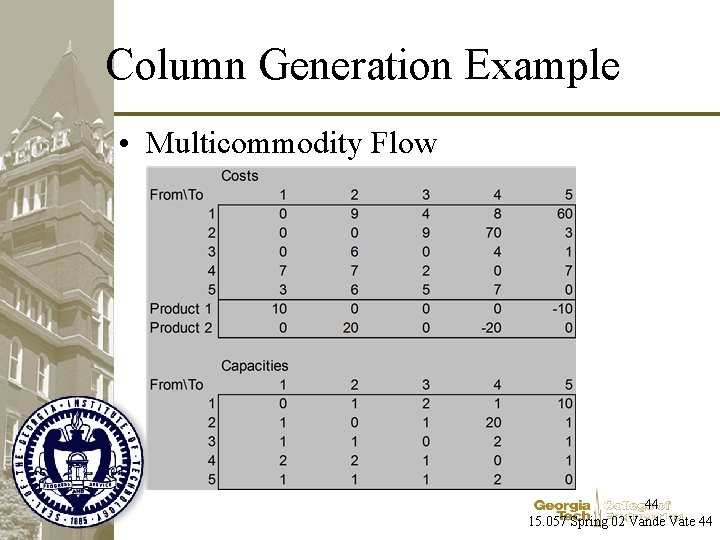
Column Generation Example • Multicommodity Flow 44 15. 057 Spring 02 Vande Vate 44

AMPL Commands • In AMPL Column. Generation. mod • Modeling languages do more than model. • They also drive the solver. 45 15. 057 Spring 02 Vande Vate 45

Summary • Conserve Flow at lowest level of detail • Distinction between transloading and container handling • Involves additional information in “Edges”, e. g. , what port it passed through • Extreme cases: Additional information is the entire path • Very Technical: Column Generation can handle these cases (sometimes). 46 15. 057 Spring 02 Vande Vate 46