Modeling compositional data Some collaborators Deformations Paul Sampson

Modeling compositional data

Some collaborators Deformations: Paul Sampson Wendy Meiring, Doris Damian Space-time: Tilmann Gneiting Francesca Bruno Deterministic models: Montserrat Fuentes, Peter Challenor Markov random fields: Finn Lindström Wavelets: Don Percival Brandon Whitcher, Peter Craigmile, Debashis Mondal

Background NAPAP, 1980’s Workshop on biological monitoring, 1986 Dirichlet process: Gary Grunwald, 1987 Current framework: Dean Billheimer, 1995 Other co-workers: Adrian Raftery, Mariabeth Silkey, Eun-Sug Park

Compositional data Vector of proportions Proportion of taxes in different categories Composition of rock samples Composition of biological populations Composition of air pollution
 0 0")
The triangle plot 1 Proportion 1 (0. 55, 0. 15, 0. 30) 0 0 Proportion 2 1 0 Proportion 3 1

The spider plot 0. 2 0. 4 0. 6 0. 8 1. 0 (0. 40, 0. 20, 0. 10, 0. 05, 0. 25)

An algebra for compositions Perturbation: For define The composition zero, so. acts as a Set Finally define so . .

The logistic normal If we say that z is logistic normal, in short Z ~ LN(m, ). Other distributions on the simplex: Dirichlet — ratios of independent gammas “Danish” — ratios of independent inverse Gaussian Both have very limited correlation structure.

Scalar multiplication Let a be a scalar. Define is a complete inner product space, with inner product given, e. g. , by N is the multinomial covariance N=I+jj. T j is a vector of k-1 ones. is a norm on the simplex. The inner product and norm are invariant to permutations of the components of the composition.
. Regression: centered covariate compositions Correspondence")
Some models Measurement error: where ej ~ LN(0, ). Regression: centered covariate compositions Correspondence in Euclidean space: xj x g uj

Some regression lines
")
Time series (AR 1)

A source receptor model Observe relative concentration Yi of k species at a location over time. Consider p sources with chemical profiles qj. Let ai be the vector of mixing proportions of the different sources at the receptor on day i. Q ~ LN, ai ~ indep LN, ei ~ zero mean LN

Juneau air quality 50 observations of relative mass of 5 chemical species. Goal: determine the contribution of wood smoke to local pollution load. Prior specification: Inference by MCMC.

Wood smoke contribution 95% CL 50% CL
 (benzo(a)) (fluoranthene) (chrysene) (benzo(b))")
Source profiles (pyrene) (benzo(a)) (fluoranthene) (chrysene) (benzo(b))
")
State-space model Space-time model of proportions State-space model: zj unobservable composition ~ LN(mj, j) yj k-vector of counts ~ Mult( Inference using MCMC again

Stability of arthropod food webs Omnivory thought to destabilize ecological communities Stability: Capacity to recover from shock (relative abundance in trophic classes) Mount St. Helens experiment: 6 treat-ments in 2 -way factorial design; 5 reps. §Predator manipulation (3 levels) §Vegetation disturbance (2 levels) Count anthropods, 6 wks after treatment. Divide into specialized herbivores, general herbivores, predators.

Specification of structure is generated from independent observations at each treatment mean depends only on treatment


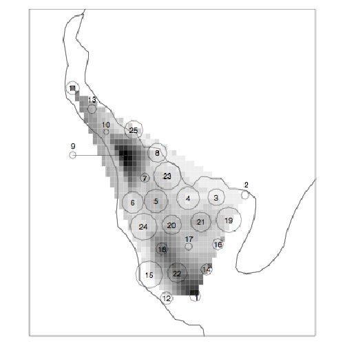
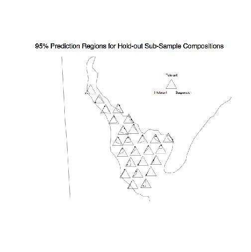
Benthic invertebrates in estuary EMAP estuaries monitoring program: Delaware Bay 1990. 25 locations, 3 grab samples of bottom sediment during summer Invertebrates in samples classified into –pollution tolerant –pollution intolerant –suspension feeders (control group; mainly palp worms)

Site j, subsample t qj ~ CAR process

Effect of salinity


- Slides: 30