Modeling Approaches to Multiple Isothermal Stability Studies for

Modeling Approaches to Multiple Isothermal Stability Studies for Estimating Shelf Life Oscar Go, Areti Manola, Jyh-Ming Shoung and Stan Altan Non-Clinical Statistics

Contents § Overview of Statistical Aspect of Stability Study § Accelerated Stability Study § Bayesian Methods § Case Study § Concluding Remarks 2

Purpose of Stability Testing § To provide evidence on how the quality of a drug substance or drug product varies with time under the influence of a variety of environmental factors (such as temperature, humidity, light, package) § To establish a re-test period for the drug substance or an expiration date (shelf life) for the drug product § To recommend storage conditions 3

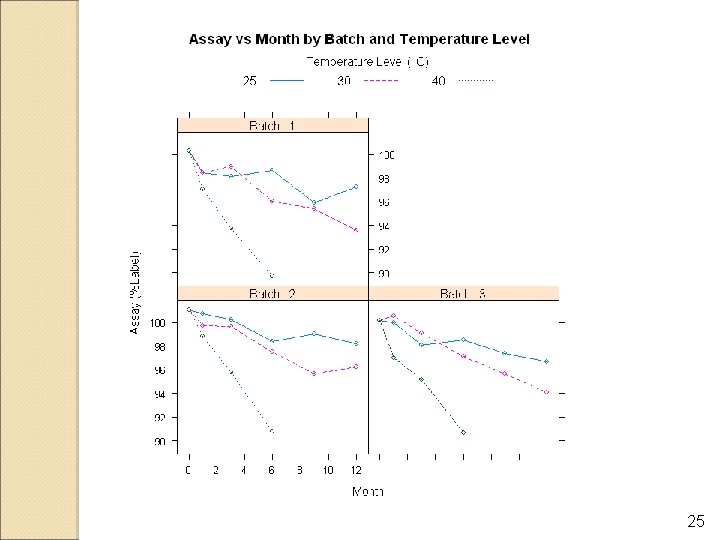
Typical Design § Randomly select containers/dosage units at time of manufacture, minimum of 3 batches, stored at specified conditions. § At specified times 0, 1, 3, 6, 9, 12, 18, 24, 36, 48, 60 months, randomly select dosage units and perform assay on composite samples § Basic Factors : Batch, Strength, Storage Condition, Time, Package § Additional Factors: Position, Drug Substance Lot, Supplier, Manufacturing Site 4

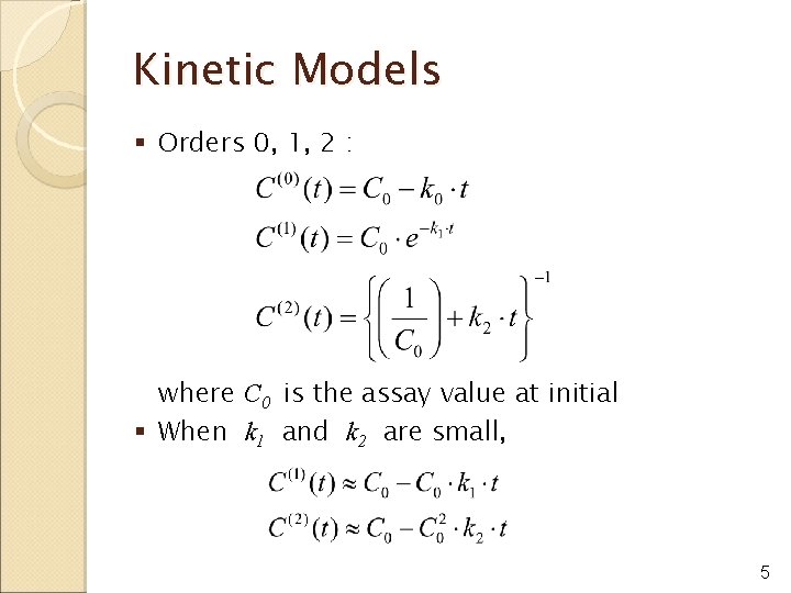
Kinetic Models § Orders 0, 1, 2 : where C 0 is the assay value at initial § When k 1 and k 2 are small, 5

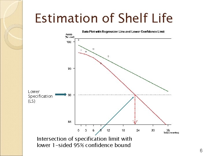
Estimation of Shelf Life Lower Specification (LS) Intersection of specification limit with lower 1 -sided 95% confidence bound 6

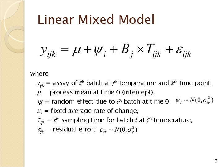
Linear Mixed Model where yijk = assay of ith batch at jth temperature and kth time point, = process mean at time 0 (intercept), i = random effect due to ith batch at time 0: Bj = fixed average rate of change, Tijk = kth sampling time for batch i at jth temperature, ijk = residual error: 7

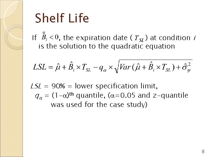
Shelf Life If , the expiration date ( TSL ) at condition i is the solution to the quadratic equation LSL = 90% = lower specification limit, q = (1 - )th quantile, ( =0. 05 and z-quantile was used for the case study) 8

Accelerated Stability Testing § Product is subjected to stress conditions. § Temperature and humidity are the most common stress factors. § Purpose is to predict long term stability and shelf life. § Arrhenius equation captures the kinetic relationship between rates and temperature. The usual fixed and mixed models ignore any relationship between rate and temperature. 9

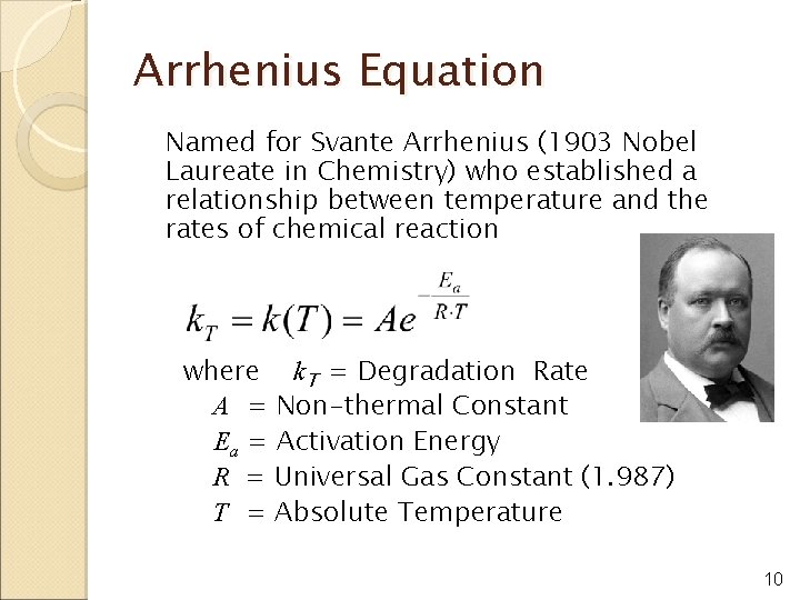
Arrhenius Equation Named for Svante Arrhenius (1903 Nobel Laureate in Chemistry) who established a relationship between temperature and the rates of chemical reaction where k. T = Degradation Rate A = Non-thermal Constant Ea = Activation Energy R = Universal Gas Constant (1. 987) T = Absolute Temperature 10

Assumptions Underlying Arrhenius Approach § The kinetic model is valid and applies to the molecule under study § Homogeneity in analytical error NB: Humidity is not acknowledged in the equation 11

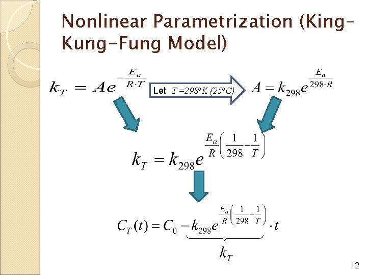
Nonlinear Parametrization (King. Kung-Fung Model) Let T =298 o. K (25 o. C) 12

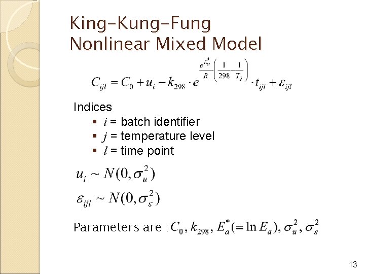
King-Kung-Fung Nonlinear Mixed Model Indices § i = batch identifier § j = temperature level § l = time point Parameters are : 13

King-Kung-Fung Model. Estimation of Shelf Life Shelf life at a given temperature Tj = T is the solution t. SL in the following equation where t 0. 95, df is the Student’s 95 th t-quantile with df degrees 14

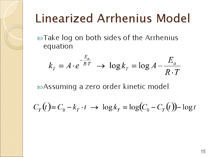
Linearized Arrhenius Model Take log on both sides of the Arrhenius equation Assuming a zero order kinetic model 15

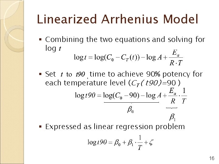
Linearized Arrhenius Model § Combining the two equations and solving for log t § Set t to t 90 , time to achieve 90% potency for each temperature level (CT ( t 90 )=90 ) § Expressed as linear regression problem 16

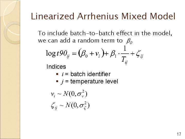
Linearized Arrhenius Mixed Model To include batch-to-batch effect in the model, we can add a random term to b 0 Indices § i = batch identifier § j = temperature level 17

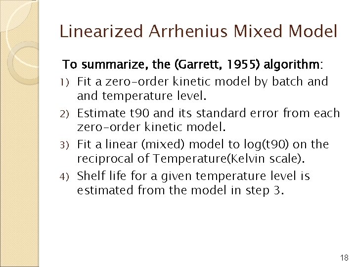
Linearized Arrhenius Mixed Model To summarize, the (Garrett, 1955) algorithm: 1) Fit a zero-order kinetic model by batch and temperature level. 2) Estimate t 90 and its standard error from each zero-order kinetic model. 3) Fit a linear (mixed) model to log(t 90) on the reciprocal of Temperature(Kelvin scale). 4) Shelf life for a given temperature level is estimated from the model in step 3. 18

Comparison Between the Three Approaches § Linear Mixed Model q Loses information contained in the Arrhenius relationship when it is valid § Linearized Arrhenius Model (Garrett) q Simple and does not require specialized software q Not clear how to estimate shelf life in relation to ICH guideline q Ignores heteroscedasticity in the error terms q Difficult to interpret the random effect § Nonlinear Model (King-Kung-Fung) q Computationally intensive q Computing convergence issues 19

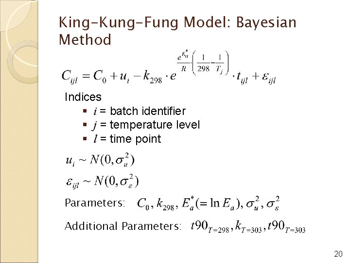
King-Kung-Fung Model: Bayesian Method Indices § i = batch identifier § j = temperature level § l = time point Parameters: Additional Parameters: 20

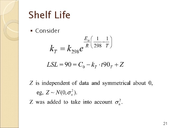
Shelf Life § Consider 21

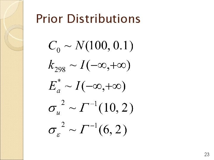
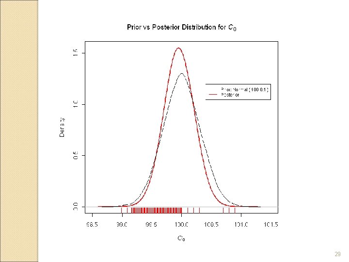
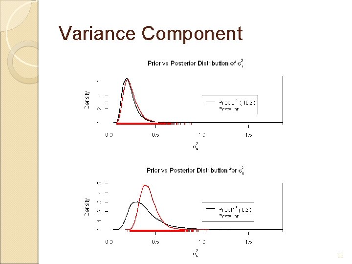
King-Kung-Fung Model: Bayesian Method-Prior Distributions § Provides a flexible framework for incorporating scientific and expert judgment, incorporating past experience with similar products and processes § Expert opinions q q q Process mean at time 0 is between 99% and 101% No information regarding degradation rate No information regarding activation energy Batch variability is between 0. 1 and 0. 5 with 99% probability Analytical variability is between 0. 1 to 1. 0 with 99% probability 22

Prior Distributions 23

Case Study 24

25

R/Win. BUGS Simulation Parameters § 3 chains § 500, 000 iterations/chain § Discard 1 st 100, 000 simulated values in each chain § Retain every 100 th simulation draw § A total of 27, 000 simulated values for each parameter 26

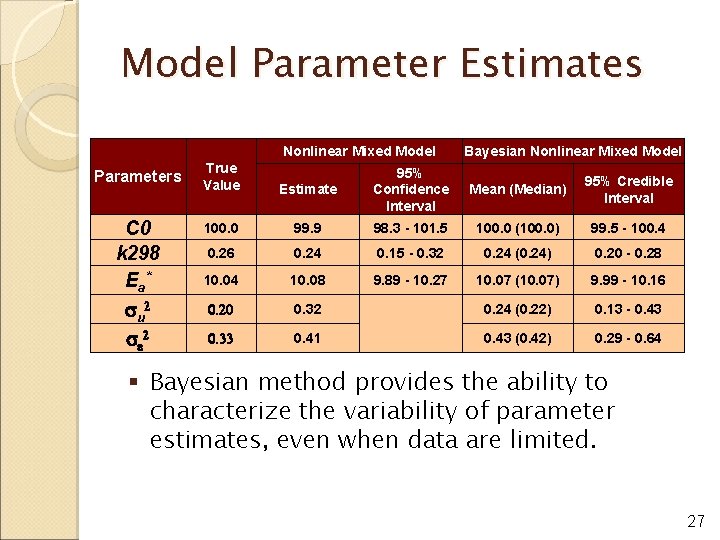
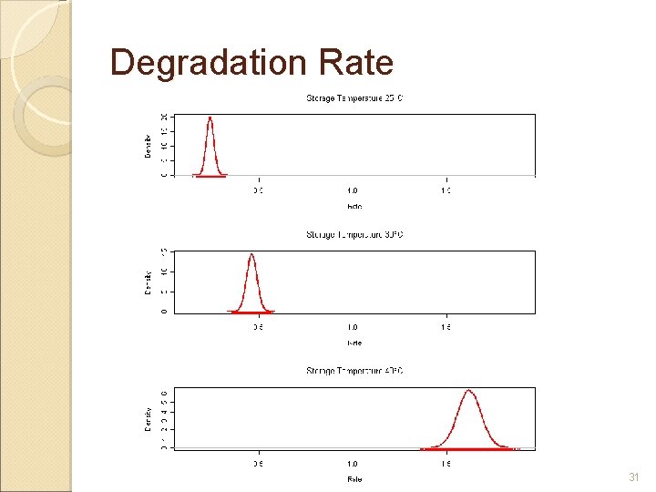
Model Parameter Estimates Nonlinear Mixed Model Parameters C 0 k 298 Ea * su 2 se 2 True Value Bayesian Nonlinear Mixed Model Estimate 95% Confidence Interval Mean (Median) 95% Credible Interval 100. 0 99. 9 98. 3 - 101. 5 100. 0 (100. 0) 99. 5 - 100. 4 0. 26 0. 24 0. 15 - 0. 32 0. 24 (0. 24) 0. 20 - 0. 28 10. 04 10. 08 9. 89 - 10. 27 10. 07 (10. 07) 9. 99 - 10. 16 0. 20 0. 32 0. 24 (0. 22) 0. 13 - 0. 43 0. 33 0. 41 0. 43 (0. 42) 0. 29 - 0. 64 § Bayesian method provides the ability to characterize the variability of parameter estimates, even when data are limited. 27

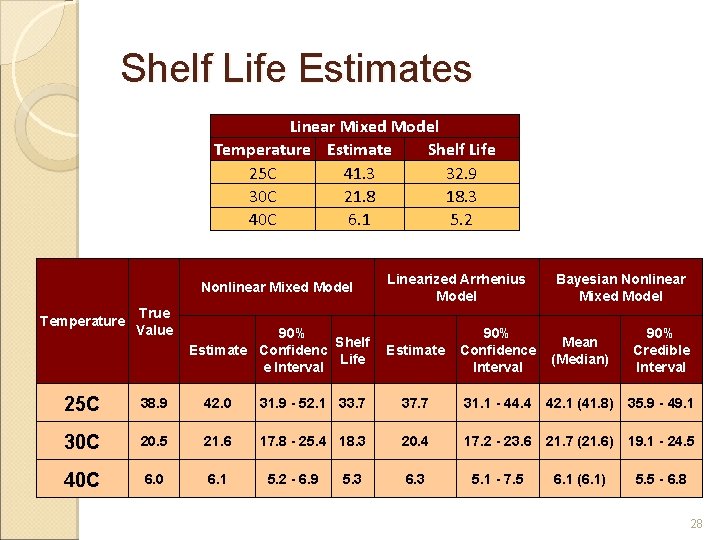
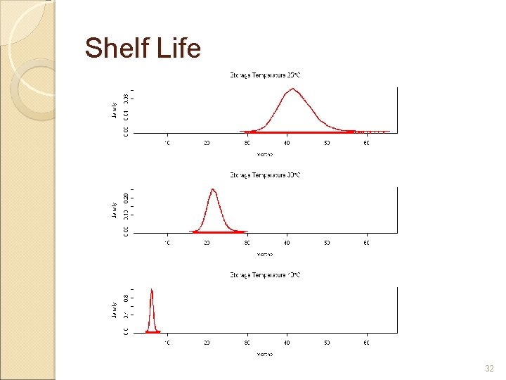
Shelf Life Estimates Linear Mixed Model Temperature Estimate Shelf Life 25 C 41. 3 32. 9 30 C 21. 8 18. 3 40 C 6. 1 5. 2 Nonlinear Mixed Model Linearized Arrhenius Model Bayesian Nonlinear Mixed Model Temperature True Value 25 C 38. 9 42. 0 31. 9 - 52. 1 33. 7 37. 7 31. 1 - 44. 4 42. 1 (41. 8) 35. 9 - 49. 1 30 C 20. 5 21. 6 17. 8 - 25. 4 18. 3 20. 4 17. 2 - 23. 6 21. 7 (21. 6) 19. 1 - 24. 5 40 C 6. 0 6. 1 6. 3 5. 1 - 7. 5 6. 1 (6. 1) 5. 5 - 6. 8 90% Shelf Estimate Confidenc Estimate Life e Interval 5. 2 - 6. 9 5. 3 90% Mean Confidence (Median) Interval 90% Credible Interval 28

29

Variance Component 30

Degradation Rate 31

Shelf Life 32

Summary § King-Kung-Fung model is a practical way to characterize multiple isothermal stability profiles and has been shown to be extended easily to a nonlinear mixed model context. § Bayesian method permits integration of expert scientific judgment in characterizing the stability property of a pharmaceutical compound. § The Bayesian credible interval can be interpreted in a probabilistic way and provides a more natural meaning to shelf life compared with the frequentist repeated sampling definition. § The problem of determining the appropriate degrees of freedom in mixed modeling is eliminated by Bayesian method. § Bayesian method is flexible and can be easily applied to a wide family of distributions. 33