Modeling and Analysis Techniques in Systems Biology CS

Modeling and Analysis Techniques in Systems Biology. CS 6221 Lecture 2 P. S. Thiagarajan

Acknowledgment • Many of the PDF images that appear in the slides to follow are taken from the text book “Systems Biology in Practice” by E. Klipp et. al.

The Role of Chemical Reactions Bio-Chemical reactions A network of Bio-Chemical reactions Interacting Bio-Chemical networks Metabolic pathways Signaling pathways Gene regulatory networks Cell functions 3

The Role of Chemical Reactions Reaction kinetics Bio-Chemical reactions A network of Bio-Chemical reactions Interacting Bio-Chemical networks Metabolic pathways Signaling pathways Gene regulatory networks Cell functions 4

Rate Laws • Rate law: – An equation that relates the concentrations of the reactants to the rate. • Differential equations are often used to describe these laws. • Assumption: The reactants participating in the reactions are abundant. 5

Reaction Kinetics • Kinetics: – Determine reaction rates q Fix reaction law and q determine reaction rate constant q Solve the equation capturing the dynamics. • The reaction rate for a product or reactant in a particular reaction: – the amount (in moles or mass units) per unit time per unit volume that is formed or removed. 6

Rate Laws • Mass action law: – The reaction rate is proportional to the probability of collision of the reactants – Proportional to the concentration of the reactants to the power of their molecularities. 7

Mass action law S 1 + S 2 V P V = k. [S 1] [S 2] [S 1] is the concentration (Moles/ litre) of S 1 [S 2] is the concentration (Moles/ litre) of S k is the rate constant V, the rate of the reaction 8

Mass-action Kinetics k 1 E+S ES k 2 k 3 E+P 9

10

• Assuming mass law kinetics we can write down a system of ordinary differential equations for the 6 species. • But we don’t know how to solve systems of ordinary (non-linear) differential equations even for dimension 4! • We must resort to numerical integration. 11

Given: 12

Initial values chosen “randomly” 13

Michaelis-Menton Kinetics • Describes the rate of enzyme-mediated reactions in an amalgamated fashion: – Based on mass action law. – Subject to some assumptions • Enzymes – Protein (bio-)catalysts • Catalyst: – A substance that accelerates the rate of a reaction without being used up. – The speed-up can be enormous! 14

Enzymes • Substrate binds temporarily to the enzyme. – Lowers the activation energy needed for the reaction. • The rate at which an enzyme works is influenced by: – concentration of the substrate – Temperature q beyond a certain point, the protein can get denatured Ø Its 3 dimensional structure gets disrupted 15

Enzymes • The rate at which an enzyme works is influenced by: – The presence of inhibitors q molecules that bind to the same site as the substrate (competitive) Ø prevents the substrate from binding q molecules that bind to some other site of the enzyme but reduces its catalytic power (non-competitive) – p. H (the concentration of hydrogen ions in a solution) q affects the 3 dimensional shape 16

Michaelis-Menton Kinetics k 1 E+S ES k 2 i) k 3 E+P A reversible formation of the Enzyme-Substrate complex ES ii) Irreversible release of the product P from the enzyme. This is for a single substrate; no backward reaction or negligible if we focus on the initial phase of the reaction. 17

Michaelis-Menten Kinetics 18

Michaelis-Menton Kinetics k 1 E+S ES k 2 k 3 E+P Use mass action law to model each reaction. 19

(1) This is the rate at which P is being produced. Assumption 1: [ES] concentration changes much more slowly than those of [S] and [P] (quasi-steady-state) We can then write: 20

This simplifies to: (2) 21

Michaelis-Menton Kinetics (1) (2) Define (Michaelis constant) (3) 22

Assumption 1: [ES] concentration changes much more slowly than those of [S] and [P] (quasi-steady-state) Assumption 2: The total enzyme concentration does not change with time. [E 0] = [E] + [ES] [E 0] - initial concentration 23

Michaelis-Menton Kinetics 24

Michaelis-Menton Kinetics (1) 25

Michaelis-Menton Kinetics Vmax is achieved when all of the enzyme (E 0) is substrate-bound. (assumption: [S] >> [E 0]) at maximum rate, Thus, 26

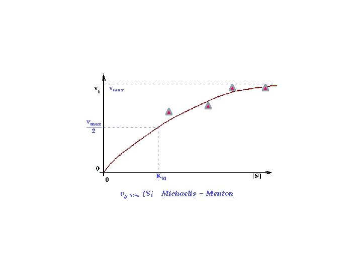
Michaelis-Menton Kinetics This is the Michaelis-Menten equation! 27

Michaelis-Menton Kinetics This is the Michaelis-Menten equation! So what? 28

Michaelis-Menton Kinetics Consider the case: The KM of an enzyme is therefore the substrate concentration at which the reaction occurs at half of the maximum rate. 29

Michaelis-Menton Kinetics 30

Michaelis-Menton Kinetics 31

Michaelis-Menton Kinetics • KM is an indicator of the affinity that an enzyme has for a given substrate, and hence the stability of the enzyme-substrate complex. • At low [S], it is the availability of substrate that is the limiting factor. • As more substrate is added there is a rapid increase in the initial rate of the reaction. 32

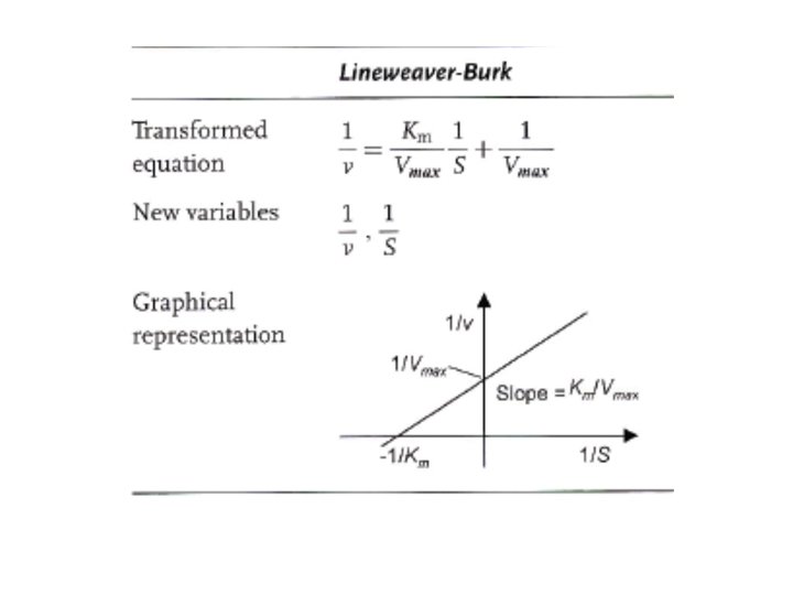
Curve Plotting • This is not relevant anymore • Good non-linear regression techniques and LARGE amounts of computing power are available.

Variations • Reversible form of Michaelis-Menten. E+S ES E+P More complicated equation but similar form.

Variations • Enzymes don’t merely accelerate reactions. • They regulate metabolism: – Their production and degradation adapted to current requirements of the cell. • Enzyme’s effectiveness targeted by inhibitors and activators (effectors).

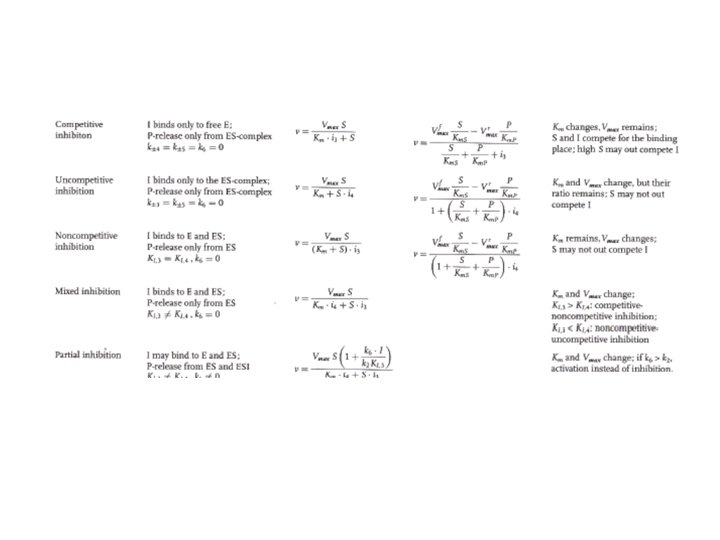
Variations • Regulatory interactions between an enzyme and an inhibitor are characterized by: – How the enzyme binds the inhibitor I q EI, ESI or both – Which complexes can release the product q ES alone or ESI or both ES and ESI

General Inhibitory Scheme

Competitive Inhibition

Competitive Inhibition S and I compete for the binding place High S may out-compete I

Uncompetitive Inhibition Inhibitor binds only to the ES complex. Does not compete but inhibits by binding elsewhere and inhibiting. S can’t out-compete I.

Other forms Inhibitions • Non-competitive inhibition • Mixed inhibition • Partial inhibition

Hill Coefficients • Suppose a dimeric (two identical sub-units linked together) protein has two identical binding sites. • The binding to the first ligand (at the first site) can facilitate binding to the second ligand. – Cooperative binding. • In general, the binding of a ligand to a macromolecule is often enhanced if there already other ligands present on the same macromolecule • The degree of cooperation is indicated by the Hill coefficient.

Hill Coefficients • A Hill coefficient of 1 indicates completely independent binding. – Independent of whether or not additional ligands are already bound. • A coefficient > 1 indicates cooperative binding. – Oxygen binding to hemoglobin: q Hill coefficient of 2. 8 – 3. 0

Hill equation Hill’s equation θ - fraction of ligand binding sites filled [L] - ligand concentration KM - ligand concentration producing half occupation (ligand concentration occupying half of the binding sites) n - Hill coefficient, describing cooperativity

Sigmoidal Plots

Summary • A bio-chemical reaction is governed by a kinetic law. – Mass law, Michalis-Menten, Hill equation, … • Different laws apply under different regimes. • Each law leads to an ODE model of the reaction kinetics. – Often, with an unknown constant of proportionality. (rate constant)

Metabolic networks: Stoichiometric network analysis

Biopathways

Metabolic Pathways • Cells require energy and material: – To grow and reproduce – Many other processes • Metabolism: – Acquire energy and use it to grow and build new cells • Highly organized process • Involves thousands of reactions catalyzed by enzymes.

Metabolic Pathways • Two types of reactions: – Catabolic: break down complex molecules to acquire energy and produce building blocks. q breakdown of food in cellular respiration – Anabolic: construct complex compounds from simpler building blocks by expending energy.

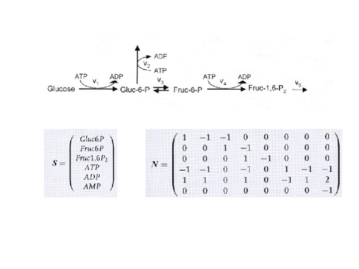
The Glycolysis Metabolic Pathway

The Glycolysis Metabolic Pathway • The individual nodes are the molecule types. • Arrows depict chemical reaction. They are labeled with the enzymes that catalyze them. • ATP and ADP play important roles.

The Glycolysis Metabolic Pathway • • ADP: Adenosine Diphosphate ATP: Adenosine Triphosphate Both nucleotides ADP ---> ATP – Energy storage (catabolic) • ATP ---> ADP – Energy release (anabolic)

Metabolic Networks • Basic constituents: – The substances with their concentrations – The (chain of) reactions and transport processes. q that change these concentrations – Reactions are usually catalyzed by enzymes – Transport carried out by transport proteins or pores.

Stoichiometric Network Analysis • Mainly used for studying metabolic networks. Properties studied: – Network consistency; blocked reactions and missing network elements – Functional pathways and cycles: “nonintutive” routes between in inputs and ouputs in complex networks; futile cycles that consume energy; inconsistent cycle consuming no energy

Stoichiometric Network Analysis • Properties studied: – Optimal pathways, sub-optimal pathways, maximal yields et. – Very useful for bio-tech applications. – Importance of single reactions for overall system performance: q knockout mutations q Enzyme deficiencies

Stoichiometric Network Analysis • Properties studied: – Correlated reactions: very likely co-regulated • Sensitivity analysis

Metabolic Networks • Stoichiometric Coefficients: – Reflect the proportion of substrate and product molecules in a reaction V 1 S 1 + S 2 2 P V 2 The stoichiometric coefficients : (-1, 2) Can also be Can even be (1, 1, -2) if the reverse reaction (V’ = V 2 – V 1) is being considered V = V 1 – V 2

Metabolic Networks • System equations • n substances and r reactions. • – i = 1, 2, …. , n - metabolites – j = 1, 2, …, r - reactions – cij = The stoichiometric coefficient of substrate (metabolite) i in the reaction j. – Vj the rates (functions of time!)

Metabolic Networks • Stoichiometric matrix –N – N(i, j) = cij

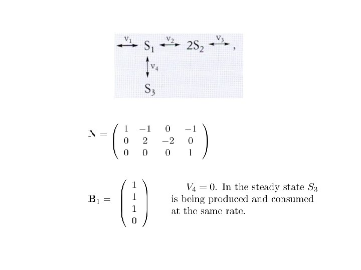
An example By convention, V 1 S 1 V 4 S 3 V 2 2 S 2 V 3 V 1 (V 2) is positive from left to right V 4 is positive from top to bottom

An example By convention, V 1 S 1 V 2 2 S 2 V 1 (V 2) is positive from left to right V 3 is positive from top to bottom V 4 S 1 S 3 S 2 S 3 V 1 V 2 V 3 V 4 1 -1 0 -1

An example By convention, V 1 S 1 V 2 2 S 2 V 1 (V 2) is positive from left to right V 3 is positive from top to bottom V 4 S 1 S 3 S 2 S 3 V 1 V 2 V 3 V 4 1 -1 0 -1 ?

An example By convention, V 1 S 1 V 2 2 S 2 V 1 (V 2) is positive from left to right V 3 is positive from top to bottom V 4 S 3 V 1 V 2 V 3 V 4 S 1 1 -1 0 -1 S 2 0 2 -1 0 S 3

An example By convention, V 1 S 1 V 2 2 S 2 V 1 (V 2) is positive from left to right V 3 P V 4 S 3 V 3 is positive from top to bottom V 1 V 2 V 3 V 4 S 1 1 -1 0 -1 S 2 0 2 -1 0 S 3

An example By convention, V 1 S 1 V 2 2 S 2 V 1 (V 2) is positive from left to right V 3 is positive from top to bottom V 4 S 3 V 1 V 2 V 3 V 4 S 1 1 -1 0 -1 S 2 0 2 -1 0 S 3 0 0 0 1

Metabolic Networks • S(t) are the functions we would like to know. – Need to solve simultaneous systems of differential equations. – Rate constants are often unknown! – Initial values not always known • Just compute the steady states.

Stoichiometric network analysis

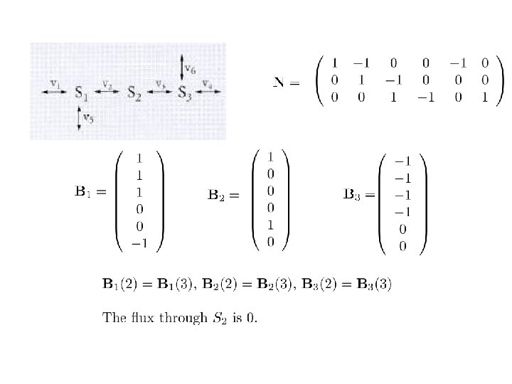
Stoichiometric Matrix Analysis • Uses only structural information. • Can compute what are the admissible fluxes possible in steady state. – Flux: The total amount of a reactant passing through (the pathway; through an enzyme; . . ) in unit time. – We are ignoring a good deal of the dynamics.

Stoichiometric network analysis

Basic linear algebra

Basic linear algebra

In steady state, the reaction rate v 8 will go to 0 ! 77

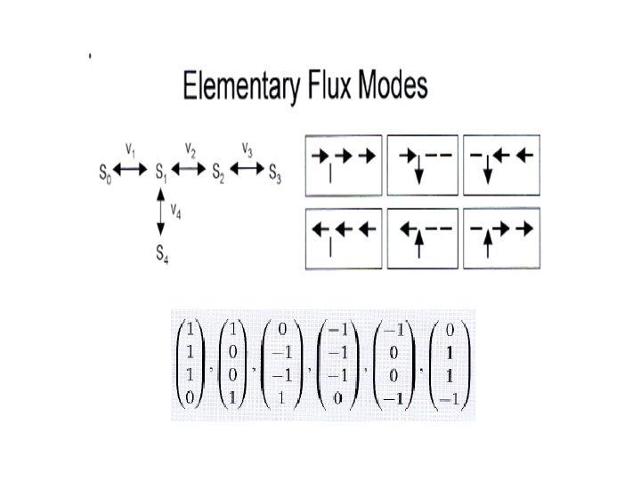
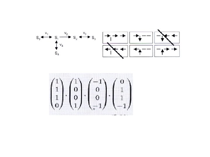
Elementary Fluxes • Elementary flux: a minimal set of non-zero -rate reactions – producing a steady state. – Respect the irreversibility (if any) of the reactions

2 1 1 0 = 1 1 + 0 1

v 2 is irreversible

Further techniques • One can do similar analysis on NT – Conserved quantities. • Quasi steady state approximations • Quasi equilibrium approximations • Replace differential equations by algebraic equations. • Sensitivity analysis (will deal with this in the context of signaling pathways)