Modeling a flexible Detector Response Function in small

Modeling a flexible Detector Response Function in small animal SPECT using Geant 4 Z. El Bitar 1, R. H. Huesman 2, R. Buchko 2, D. Brasse 1, G. T. Gullberg 2 1. Université de Strasbourg, IPHC, 23 rue du loess, 67037 Strasbourg, France 2. Lawrence Berkeley National Laboratory, Berkeley California 94720, USA 1 Droite Workshop, Lyon, October 25, 2012

Outline 1. Context 2. Fully 3 D image reconstruction 3. Monte Carlo modelling of the system matrix 4. Including geometrical misalignment 5. Correcting for penetration 6. Phantom and preclinical results 2

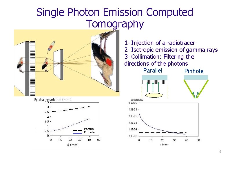
Single Photon Emission Computed Tomography 1 - Injection of a radiotracer 2 - Isotropic emission of gamma rays 3 - Collimation: Filtering the directions of the photons Parallel Pinhole 3

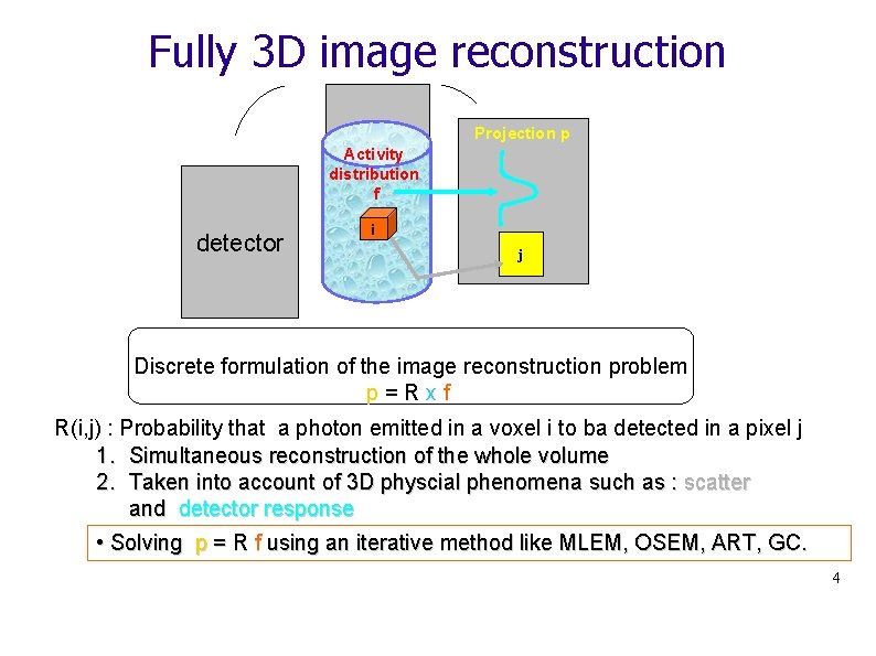
Fully 3 D image reconstruction Projection p Activity distribution f detector i j Discrete formulation of the image reconstruction problem p=Rxf R(i, j) : Probability that a photon emitted in a voxel i to ba detected in a pixel j 1. Simultaneous reconstruction of the whole volume 2. Taken into account of 3 D physcial phenomena such as : scatter and detector response • Solving p = R f using an iterative method like MLEM, OSEM, ART, GC. 4

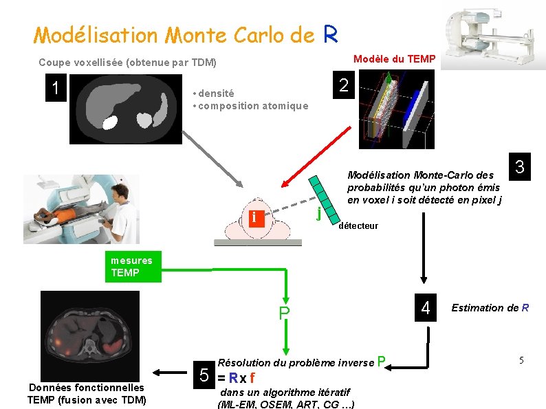
Modélisation Monte Carlo de R Modèle du TEMP Coupe voxellisée (obtenue par TDM) 1 2 • densité • composition atomique j i Modélisation Monte-Carlo des probabilités qu’un photon émis en voxel i soit détecté en pixel j 3 détecteur mesures TEMP P Données fonctionnelles TEMP (fusion avec TDM) 5 Résolution du problème inverse P = Rx f dans un algorithme itératif (ML-EM, OSEM, ART, CG …) 4 Estimation de R 5

What’s the problem in small animal SPECT ? 1. Monte Carlo simulations are time consuming. 2. Detection efficiency is very low in small animal SPECT due to pinhole collimation. 3. Pinhole SPECT modality is very sensitive to geometrical misalignments => a system matrix should be computed for each set up. 4. We must find a solution to avoid resimulation by Monte Carlo methods for each exam => need to have a detector model independent of the acquisition set up. 6

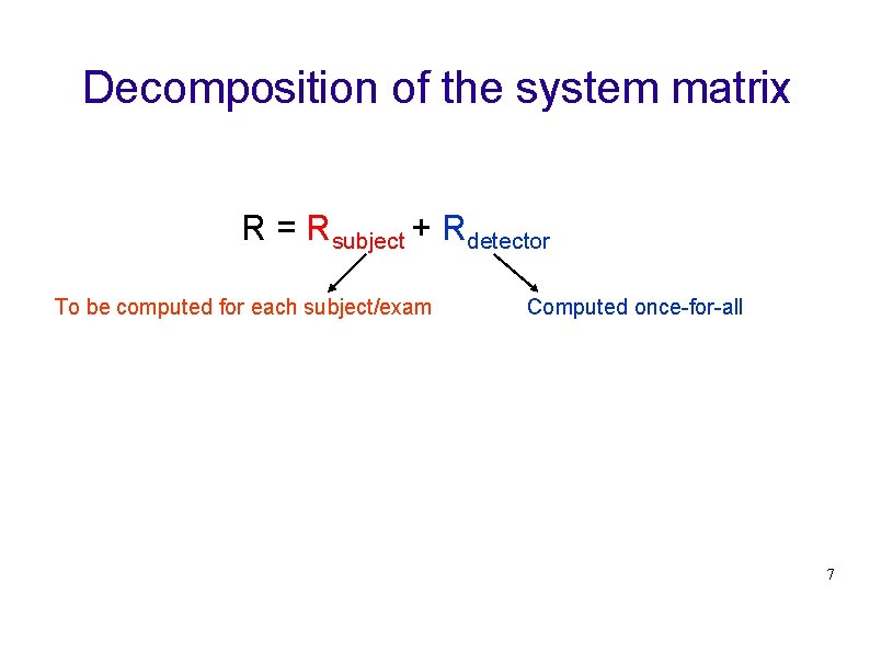
Decomposition of the system matrix R = Rsubject + Rdetector To be computed for each subject/exam Computed once-for-all 7

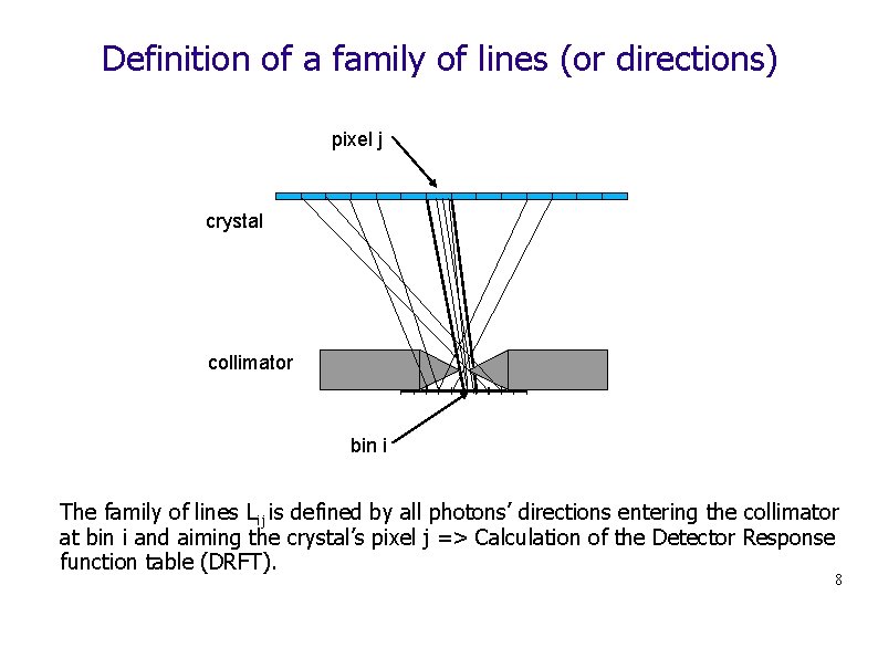
Definition of a family of lines (or directions) pixel j crystal collimator bin i The family of lines Lij is defined by all photons’ directions entering the collimator at bin i and aiming the crystal’s pixel j => Calculation of the Detector Response function table (DRFT). 8

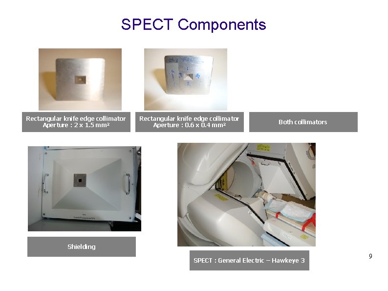
SPECT Components Rectangular knife edge collimator Aperture : 2 x 1. 5 mm 2 Rectangular knife edge collimator Aperture : 0. 6 x 0. 4 mm 2 Both collimators Shielding SPECT : General Electric – Hawkeye 3 9

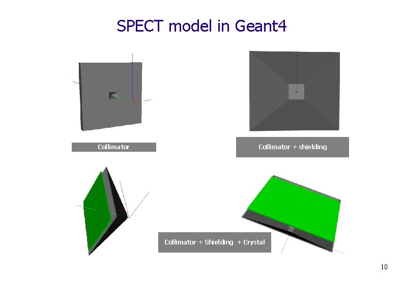
SPECT model in Geant 4 Collimator + shielding Collimator + Shielding + Crystal 10

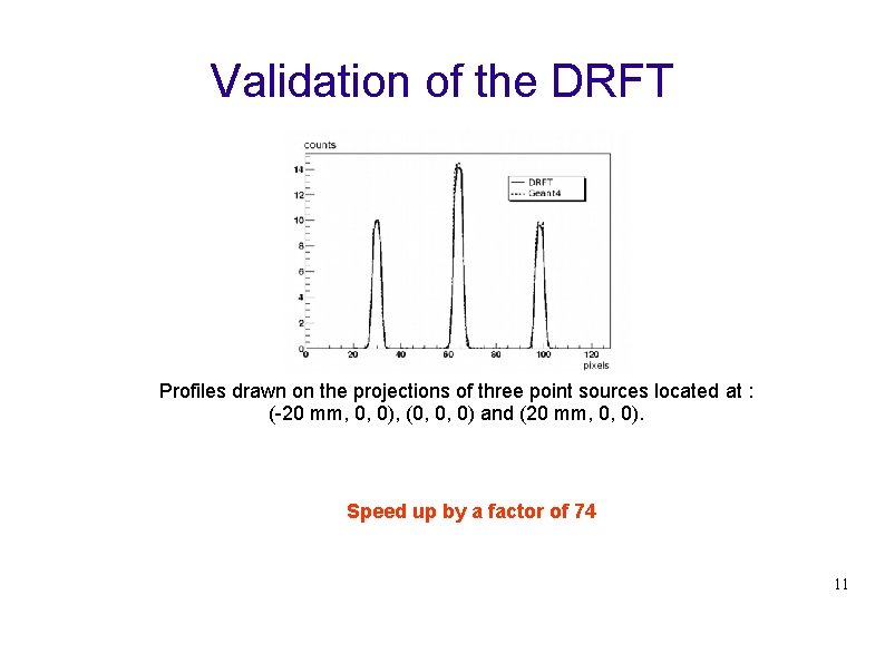
Validation of the DRFT Profiles drawn on the projections of three point sources located at : (-20 mm, 0, 0), (0, 0, 0) and (20 mm, 0, 0). Speed up by a factor of 74 11

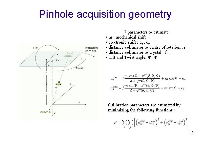
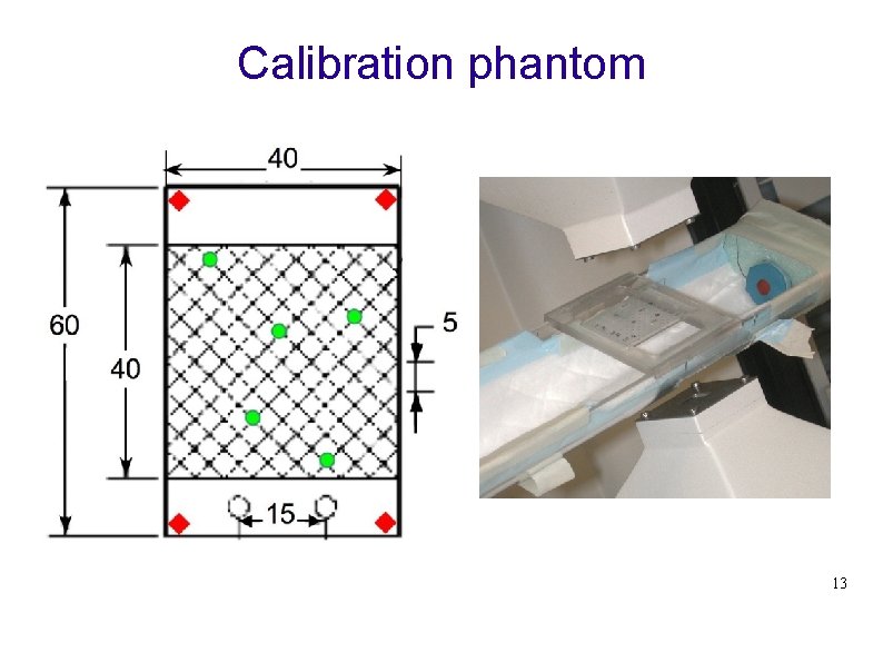
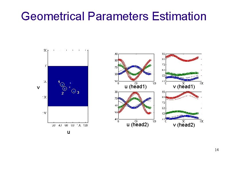
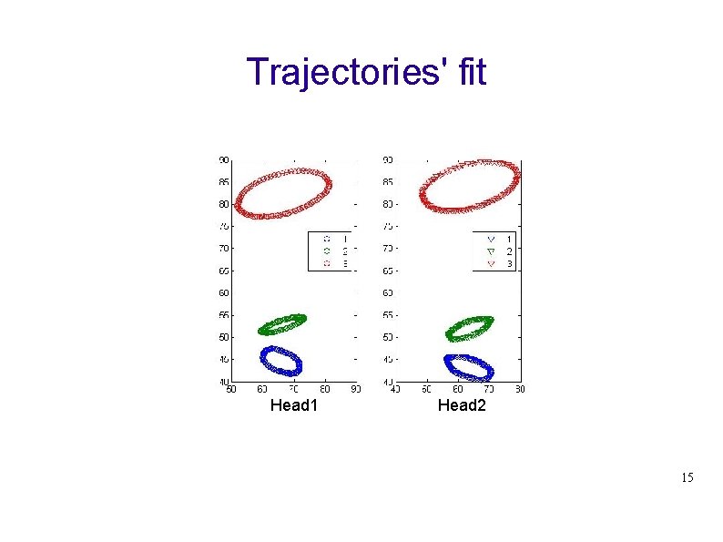
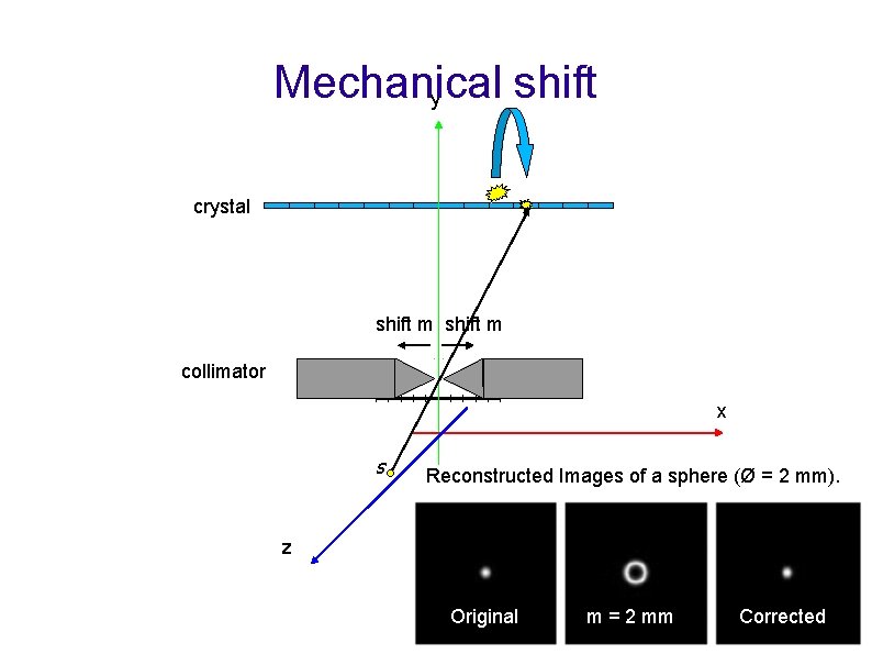
Pinhole acquisition geometry 7 parameters to estimate: • m : mechanical shift • electronic shift : eu , ev • distance collimator to centre of rotation : r • distance collimator to crystal : f • Tilt and Twist angle: Ф, Ψ Calibration parameters are estimated by minimizing the following functions : 12

Calibration phantom 1 2 3 13

Geometrical Parameters Estimation 1 u (head 1) v v (head 1) 3 2 u (head 2) v (head 2) u 14

Trajectories' fit Head 1 Head 2 15

Mechanical shift y crystal shift m collimator x s Reconstructed Images of a sphere (Ø = 2 mm). z 16 Original m = 2 mm Corrected

What’s the point ? 1. After performing Monte Carlo simulations and calculating a Detector Response Function Table, one is home-free to used the DRFT(~500 Mbytes). 2. The DRFT can incorporate with ease for any geometrical misalignments (translation, rotation): all what is required is the equation of the entry plan (collimator) and the detection plan (crystal). 3. Resimulation of all photons’ trajectories inside the detector is not required for each study. 17

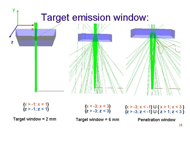
y Target emission window: x z {x > -1; x < 1} {z > -1; z < 1} {x > -3; x < 3} {z > -3; z < 3} Target window = 2 mm Target window = 6 mm {x > -3; x < -1} U { x > 1; x < 3 } {z > -3; z < -1} U { z > 1; z < 3 } Penetration window 18

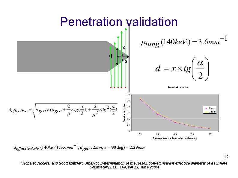
Penetration validation x d α 19 *Roberto Accorsi and Scott Metzler : Analytic Determination of the Resolution-equivalent effective diameter of a Pinhole Collimator (IEEE, TMI, vol 23, June 2004)

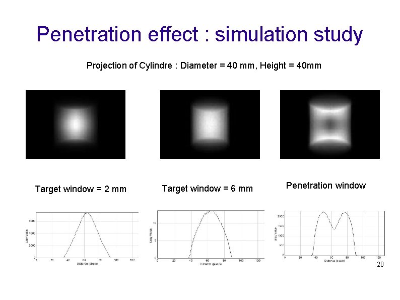
Penetration effect : simulation study Projection of Cylindre : Diameter = 40 mm, Height = 40 mm Target window = 2 mm Target window = 6 mm Penetration window 20

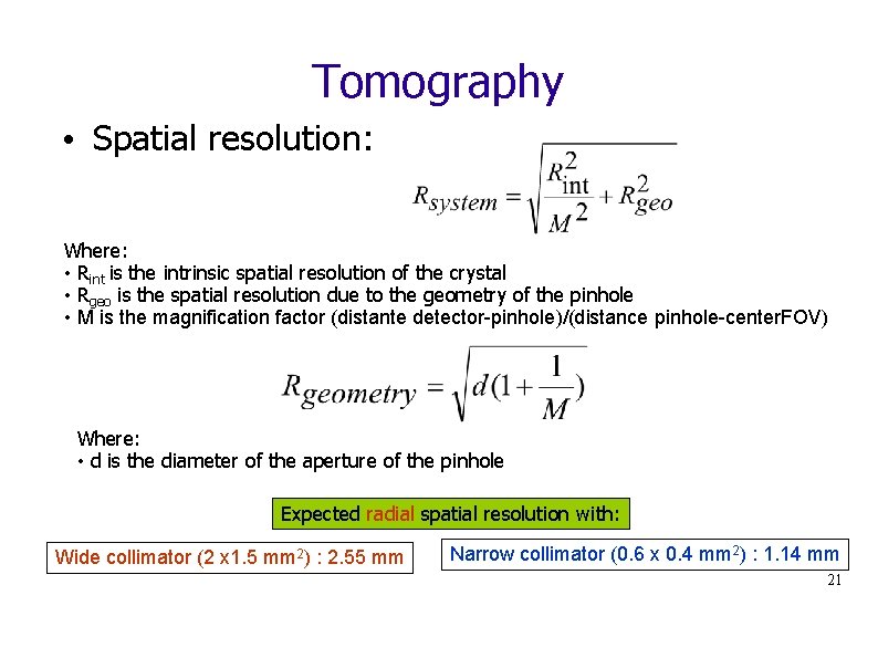
Tomography • Spatial resolution: Where: • Rint is the intrinsic spatial resolution of the crystal • Rgeo is the spatial resolution due to the geometry of the pinhole • M is the magnification factor (distante detector-pinhole)/(distance pinhole-center. FOV) Where: • d is the diameter of the aperture of the pinhole Expected radial spatial resolution with: Wide collimator (2 x 1. 5 mm 2) : 2. 55 mm Narrow collimator (0. 6 x 0. 4 mm 2) : 1. 14 mm 21

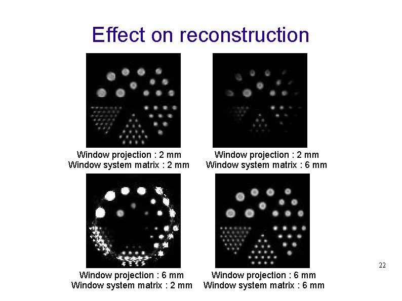
Effect on reconstruction Window projection : 2 mm Window system matrix : 2 mm Window projection : 2 mm Window system matrix : 6 mm 22 Window projection : 6 mm Window system matrix : 2 mm Window projection : 6 mm Window system matrix : 6 mm

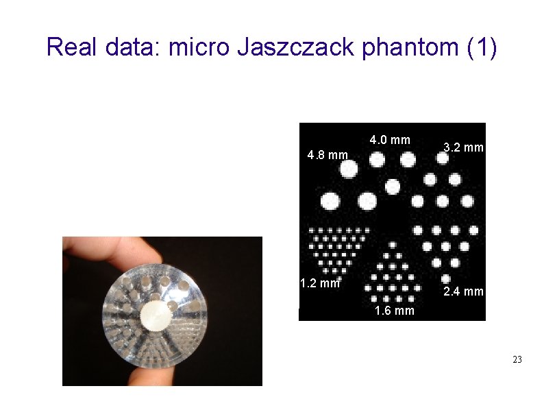
Real data: micro Jaszczack phantom (1) 4. 0 mm 4. 8 mm 1. 2 mm 3. 2 mm 2. 4 mm 1. 6 mm 23

Real data: micro Jaszczack phantom (2) 2 mm Correction for the penetration effect 1. 5 mm Window system matrix : 2 mm Window system matrix : 6 mm 24

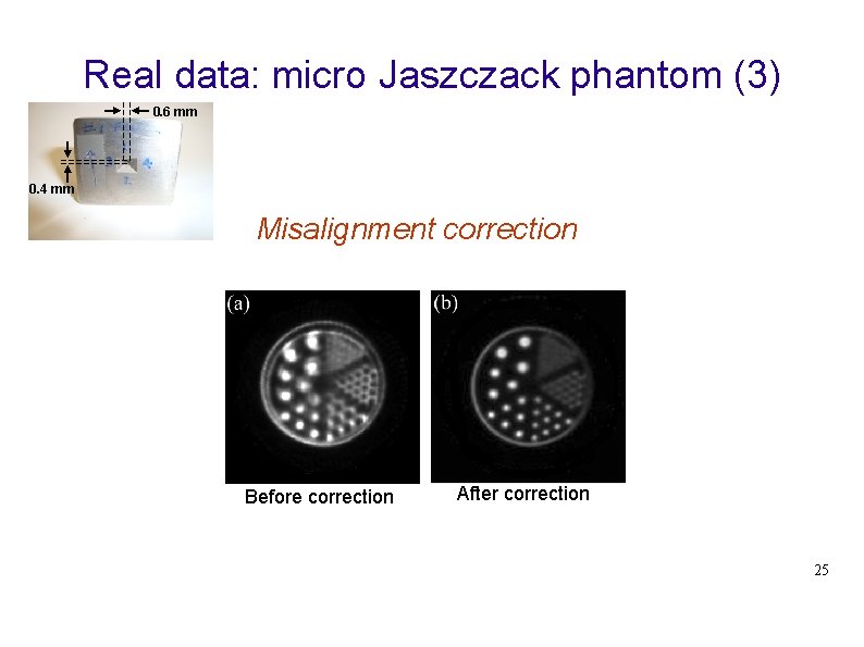
Real data: micro Jaszczack phantom (3) 0. 6 mm 0. 4 mm Misalignment correction Before correction After correction 25

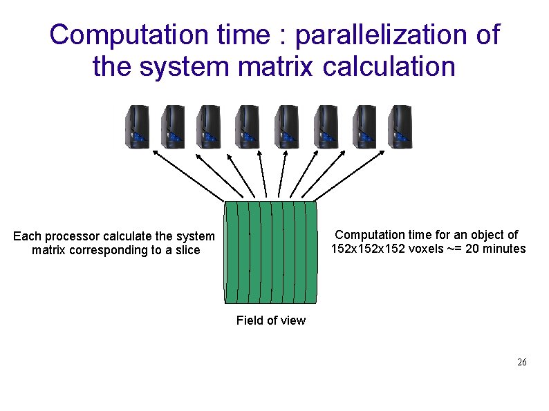
Computation time : parallelization of the system matrix calculation Computation time for an object of 152 x 152 voxels ~= 20 minutes Each processor calculate the system matrix corresponding to a slice Field of view 26

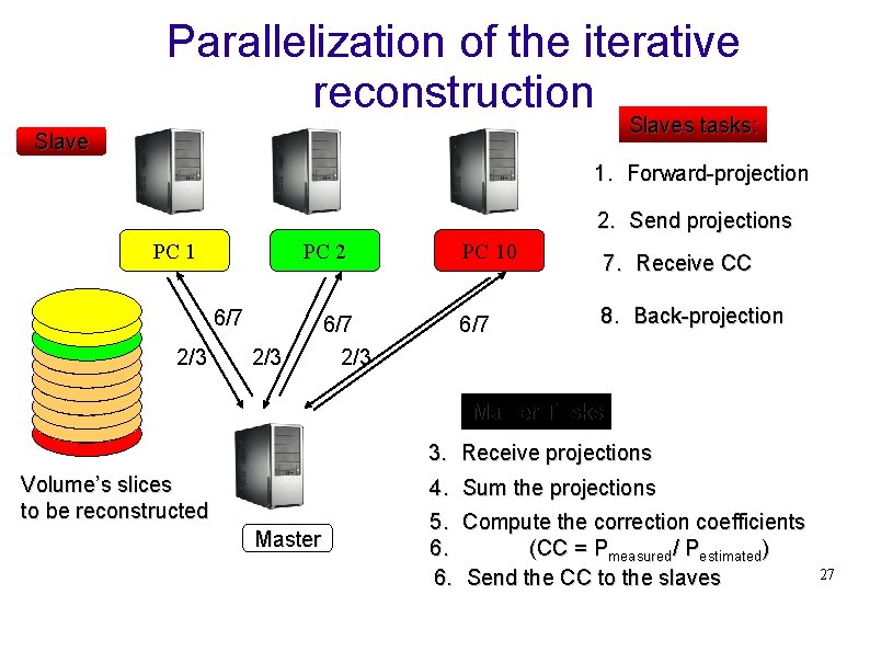
Parallelization of the iterative reconstruction Reconstruction Tomographique Slaves tasks: Slave 1. Forward-projection 2. Send projections PC 1 PC 2 6/7 2/3 PC 10 6/7 2/3 6/7 7. Receive CC 8. Back-projection Master Tasks 3. Receive projections Volume’s slices to be reconstructed Master 4. 5. 6. 6. Sum the projections Compute the correction coefficients (CC = Pmeasured/ Pestimated) Send the CC to the slaves 27

Most recent result 150 x 150 voxels (0. 4 x 0. 4 mm 3), 90 projections (128 x 88 pixels) Size of system matrix ~= 40 GBytes MLEM (50 iterations) < 3 minutes 0. 6 x 0. 4 mm 2 28

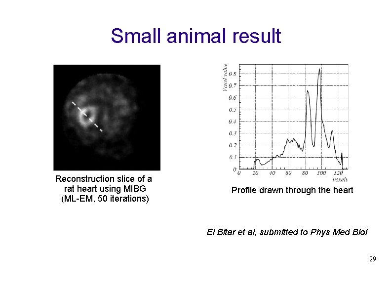
Small animal result Reconstruction slice of a rat heart using MIBG (ML-EM, 50 iterations) Profile drawn through the heart El Bitar et al, submitted to Phys Med Biol 29

Acknowledgment Grant T Gullberg (discussion) Ronald H Huesman (discussion) Rostystalv Boutchko (calibration) Archontis Giannakdis (discussion) Martin Boswell (computing) Nichlas Vandeheye (experiments) Steven Hanrahan (experiments) Bill Moses (experiments) Special thanks to the Franco-American Fulbright-commission ! 30