ModelBased Systems Design with MATLABSIMULINK Slobodan Lubura What

Model-Based Systems Design with MATLAB/SIMULINK Slobodan Lubura

What is Model-Based-System Design? • Model-Based-System Design use the models to describe the specifications, operation, performance of a component or a system of components • Instead of listing specification in a text document, a model is used that implements the specifications, operation, and performance of components

What is Model-Based-System Design? • Models can be shared with other engineers: Engineers do not have to generate their own models from text specifications. • Same model can be used by several engineers at several different levels in the design process. • Component models can be used in larger systems • Models supplied by manufacturers accurately reflect the performance of their components •

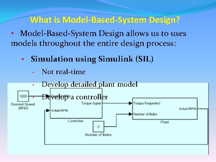
What is Model-Based-System Design? • Model-Based-System Design allows us to uses models throughout the entire design process: • Simulation using Simulink (SIL) • Not real-time • Develop detailed plant model • Develop a controller

What is Model-Based-System Design? • Real-Time Simulations: o Determine how the systems responds in real-time o Good for human-system interaction o Additional debugging • Targeting: o Implement the controller in SIL and make a Real-Time simulations on a hardware target platform (embedded controller) o Most logic errors have been removed o Errors occur if model is inaccurate

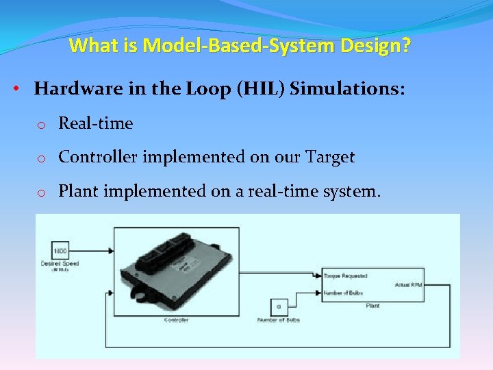
What is Model-Based-System Design? • Hardware in the Loop (HIL) Simulations: o Real-time o Controller implemented on our Target o Plant implemented on a real-time system.

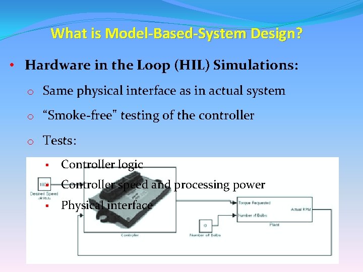
What is Model-Based-System Design? • Hardware in the Loop (HIL) Simulations: o Same physical interface as in actual system o “Smoke-free" testing of the controller o Tests: § Controller logic § Controller speed and processing power § Physical interface.

What is Model-Based-System Design? • Controller deployment: o Given accurate models and a consistent interface, we can just plug in the controller to our plant o It should work perfectly the first time!! (Not) o It should work reasonable well, but we will notice that the plant model may have inaccuracies o Typically we will need to modify the plant and controller to account for the differences.

Example: Model-Based Design of a Motor-Generator System in MATLAB/SIMULINK

Model-Based Design Solution • Create Plant and Controller Models o Motor and Generator Models o P and PI Controllers • Simulate with Simulink • Real-Time Simulations with x. PC target • Implement Controller on Microchip ds. PIC Real-Time Target or …. • Test • Improve Model and Controller • Repeat

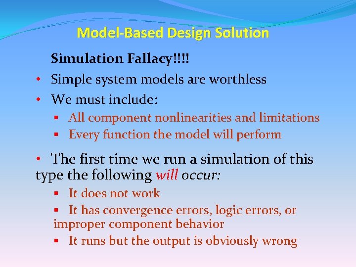
Model-Based Design Solution Simulation Fallacy!!!! • Simple system models are worthless • We must include: § All component nonlinearities and limitations § Every function the model will perform • The first time we run a simulation of this type the following will occur: § It does not work § It has convergence errors, logic errors, or improper component behavior § It runs but the output is obviously wrong

Modeling Building Philosophy • • • Start with simple component models Understand simple component operation Develop a simple controller Anticipate expected system output Verify that output matches expectation

Modeling Building Philosophy • Add a single function to the model and: § Understand the effect on the: § § § Component System Controller § Anticipate the expected system output § Verify that output matches expectation • Repeat as needed…

Model Building with Simulink - High Level System • Using the Simulink to build a model of the plant and controller: Plant : Motor, Generator, Shaft Encoder o Controller: P or PI o Plant Input : Light bulb load o Controller Input : Generator speed o • First build a very simple plant • We are aiming for the following system:

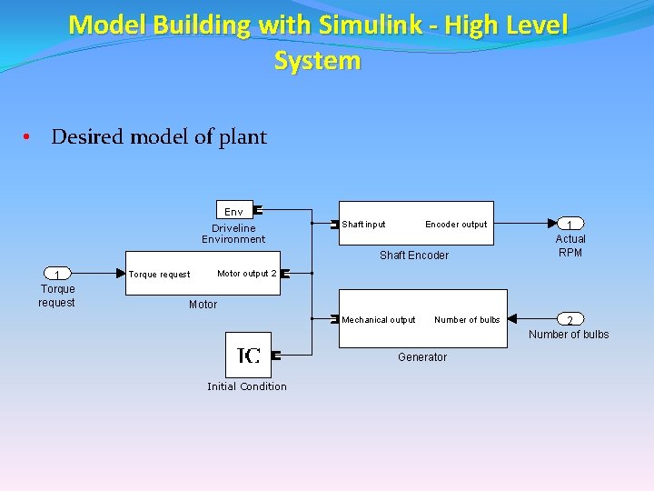
Model Building with Simulink - High Level System • Desired model of plant Env Driveline Environment Encoder output Shaft input Shaft Encoder 1 Torque request 1 Actual RPM Motor output 2 Torque request Motor Mechanical output Number of bulbs Generator Initial Condition 2 Number of bulbs

Model Building with Simulink • To build plant (and controller), we will use MBSD: o Start with simple component models o Anticipate the appropriate system responses o Verify the model works correctly o Make ONE improvement o Understand effect on model o Repeat

Model Building with Simulink- plant model • The first is created simple a model of ideal DC motor : o Variable torque from 0 to max rated value o No rpm limits o No energy conversion inefficiencies o No frictional losses o Torque is independent of rpm • This is a terribly inaccurate model, but it is an easy to understand first step

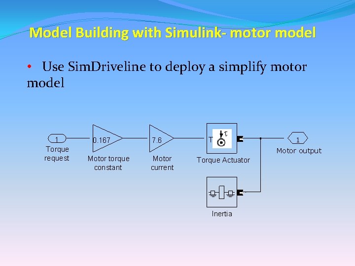
Model Building with Simulink- motor model • Use Sim. Driveline to deploy a simplify motor model 1 Torque request 0. 167 Motor torque constant 7. 6 Motor current T 1 Motor output Torque Actuator Inertia

Model Building with Simulink- improved motor model • We will improve the motor model by making the motor torque a function of motor rpm • Use a lookup table to implement the rpm dependence of the motor • Obtain a lookup table from the manufacturer data • Later on we will design an experiment and measure the actual torque curve of the motor

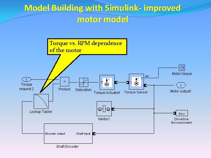
Model Building with Simulink- improved motor model Torque vs. RPM dependence of the motor Motor torque T 1 Torque request 2 T Product Saturation Torque Actuator 1 Lookup Table 1 B F Torque Sensor 1 Motor output 1 Env Inertia 1 Encoder output Shaft input Shaft Encoder Driveline Environment

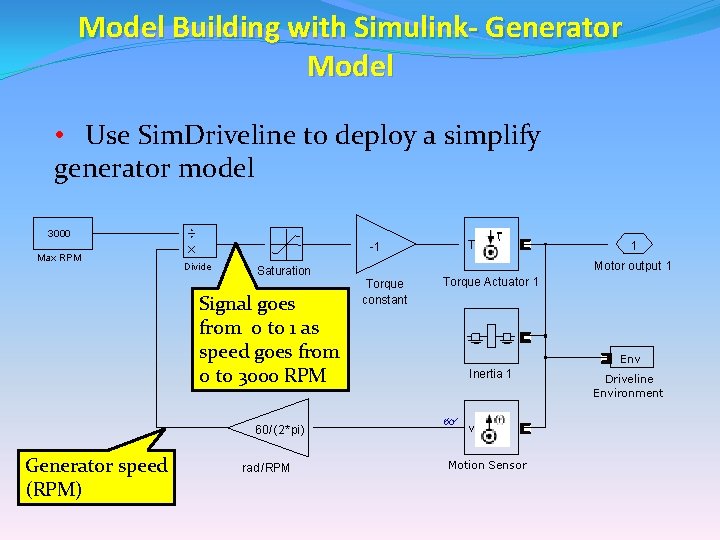
Model Building with Simulink- Generator Model • Use Sim. Driveline to deploy a simplify generator model 3000 Max RPM -1 Divide Saturation Signal goes from 0 to 1 as speed goes from 0 to 3000 RPM 60 /(2*pi) Generator speed (RPM) rad /RPM T 1 Motor output 1 Torque constant Torque Actuator 1 Env Inertia 1 v Motion Sensor Driveline Environment

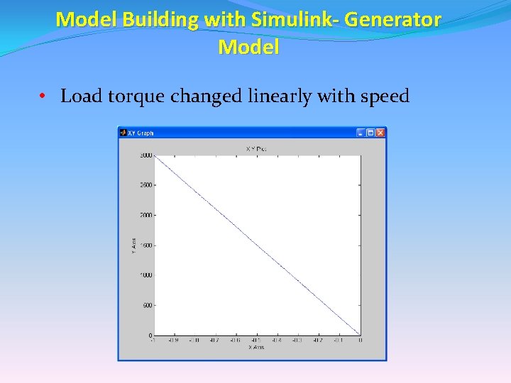
Model Building with Simulink- Generator Model • Load torque changed linearly with speed

Model Building with Simulink- improved generator model • The max load was equivalent to all of the light bulbs being turned on • The generator produces a voltage that is proportional to the generator speed. • This voltage is applied to the light bulbs, and the bulbs draw current proportional to the voltage applied across them (Ohm’s Law) • To supply the current, the generator produces a torque that opposes its direction of motion.

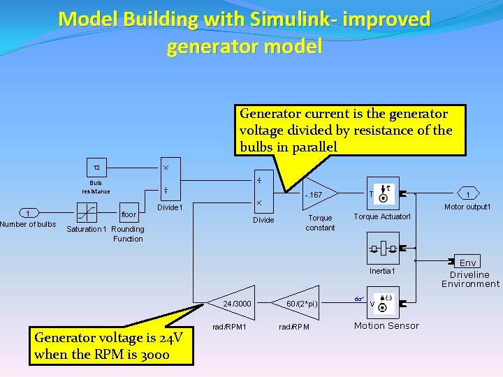
Model Building with Simulink- improved generator model Generator current is the generator voltage divided by resistance of the bulbs in parallel 12 Bulb resistance 1 Number of bulbs -. 167 floor T Motor output 1 Divide Saturation 1 Rounding Function Torque constant Torque Actuator 1 Inertia 1 24/3000 Generator voltage is 24 V when the RPM is 3000 1 rad/RPM 1 60/(2*pi) rad/RPM v Motion Sensor Env Driveline Environment

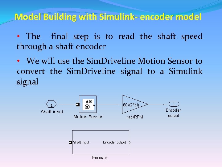
Model Building with Simulink- encoder model • The final step is to read the shaft speed through a shaft encoder • We will use the Sim. Driveline Motion Sensor to convert the Sim. Driveline signal to a Simulink signal 1 v 60 /(2*pi) Shaft input Motion Sensor Shaft input rad /RPM Encoder output Encoder 1 Encoder output

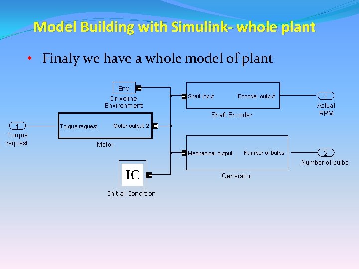
Model Building with Simulink- whole plant • Finaly we have a whole model of plant Env Driveline Environment Encoder output Shaft input Shaft Encoder 1 Torque request 1 Actual RPM Motor output 2 Torque request Motor Mechanical output Number of bulbs Generator Initial Condition 2 Number of bulbs

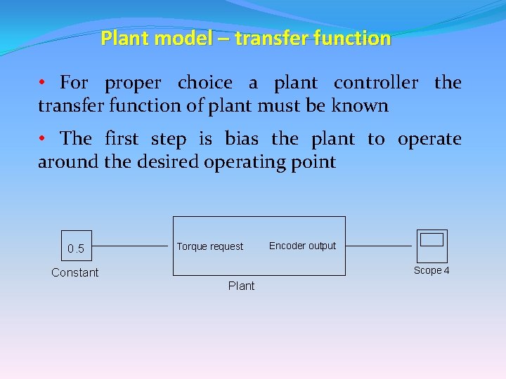
Plant model – transfer function • For proper choice a plant controller the transfer function of plant must be known • The first step is bias the plant to operate around the desired operating point 0. 5 Torque request Encoder output Scope 4 Constant Plant

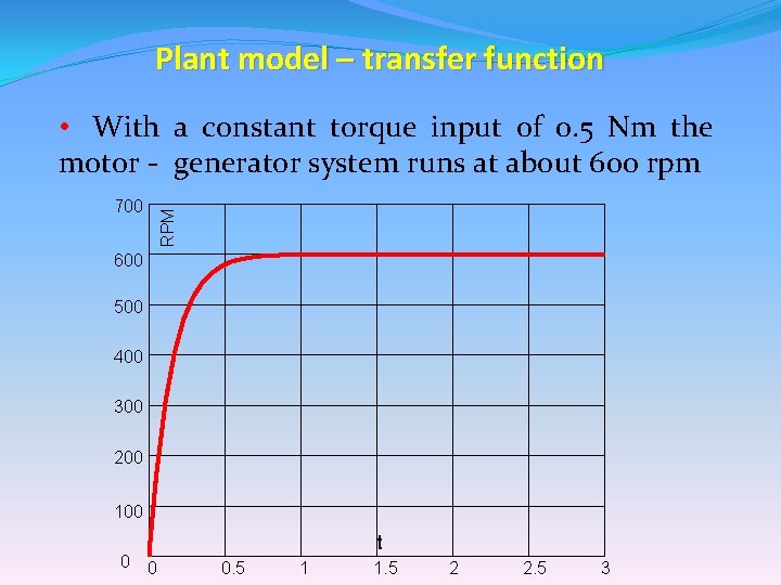
Plant model – transfer function 700 RPM • With a constant torque input of 0. 5 Nm the motor - generator system runs at about 600 rpm 600 500 400 300 200 100 0 t 0 0. 5 1 1. 5 2 2. 5 3

Plant model – transfer function • Now that we have our plant biased at 600 rpm, we will introduce a small-signal sine wave at the input and measure the magnitude of the output at various frequencies 0. 5 Constant 1 Sine Wave Torque request Encoder output Scope 4 Plant

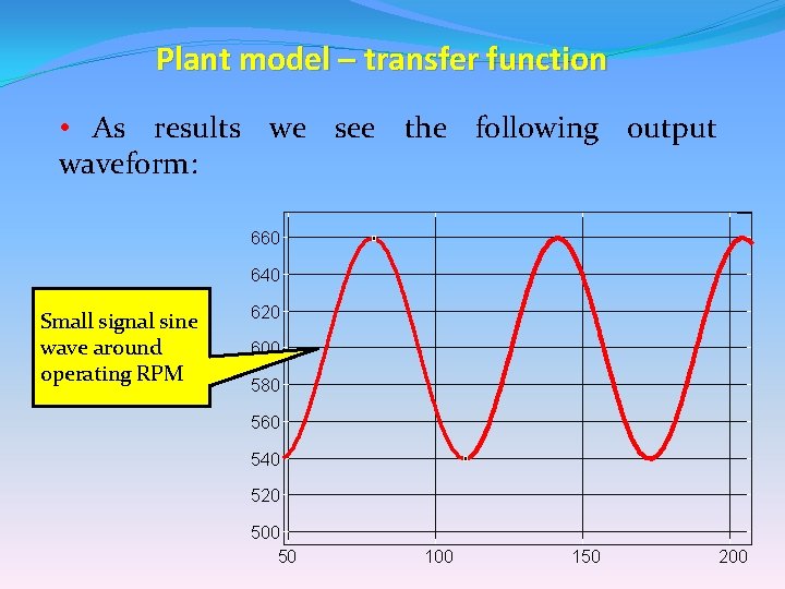
Plant model – transfer function • As results we see the following output waveform: 660 640 Small signal sine wave around operating RPM 620 600 580 560 540 520 50 100 150 200

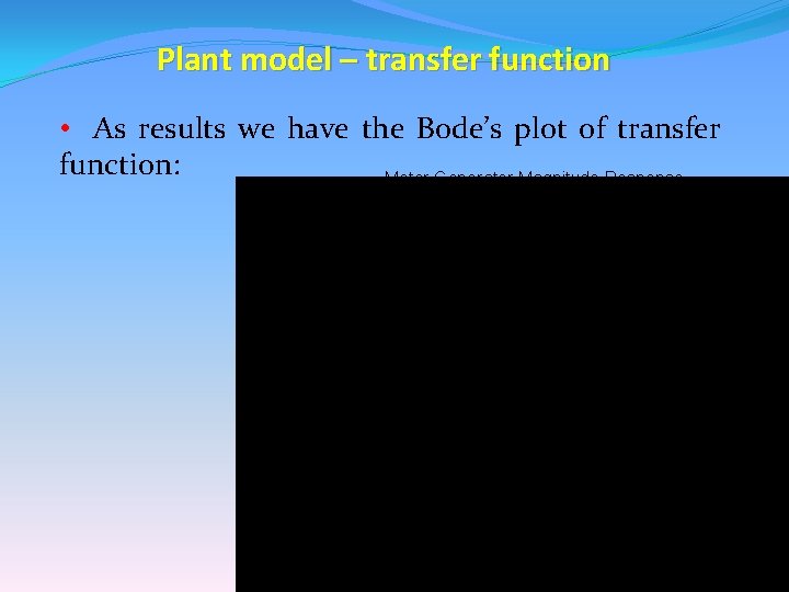
Plant model – transfer function • As results we have the Bode’s plot of transfer function: Motor Generator Magnitude Response 65 60 Amplitude (d. B) 55 50 45 40 35 30 25 -1 10 101 10 2 Frequency (rad/sec) 10 3 10 4

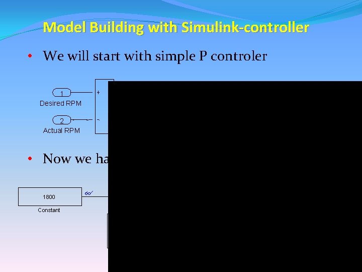
Model Building with Simulink-controller • We will start with simple P controler 1 Desired RPM 2 Actual RPM P-Gain Error amplifier Saturation 1 Out 1 • Now we have a top-level block diagram 1800 Constant Desired RPM Out 1 Actual RPM In 1 Actual RPM Controller Plant

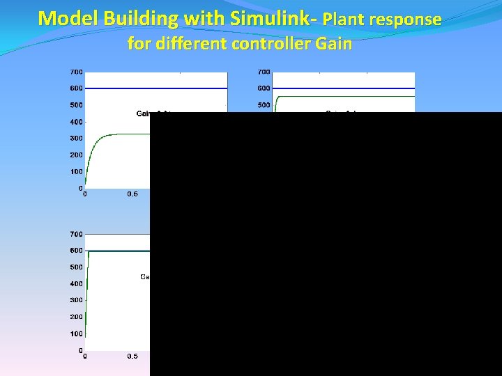
Model Building with Simulink- Plant response for different controller Gain

Model Based System design • This is why we do MBSD Understand a complex system using simple components • Understand effect of controller and components / loads on system response • Identify model improvement • shortcomings for future

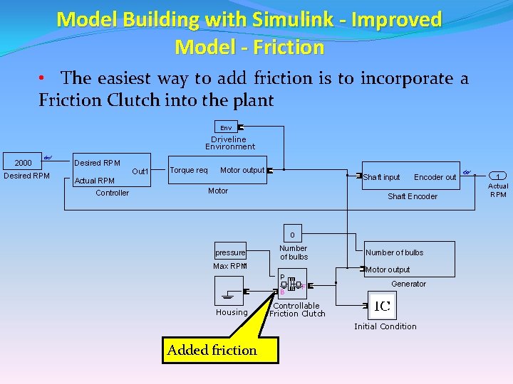
Model Building with Simulink - Improved Model - Friction • The easiest way to add friction is to incorporate a Friction Clutch into the plant Env Driveline Environment 2000 Desired RPM Out 1 Torque req Motor output Shaft input Actual RPM Controller Motor Encoder out Shaft Encoder 0 pressure 1 Max RPM Number of bulbs Motor output P B Housing Number of bulbs F Generator Controllable Friction Clutch Initial Condition Added friction 1 Actual RPM

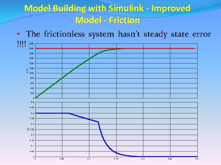
Model Building with Simulink - Improved Model - Friction • The frictionless system hasn’t steady state error !!!! 2200 2000 1800 1600 RPM 1400 1200 1000 800 600 400 200 0 0. 5 0. 4 0. 35 Nm 0. 3 0. 25 0. 2 0. 15 0. 1 0. 05 0 0 0. 05 0. 15 0. 25 0. 3

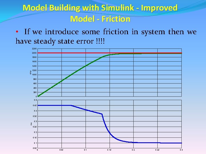
Model Building with Simulink - Improved Model - Friction • If we introduce some friction in system then we have steady state error !!!! 2200 2000 1800 1600 RPM 1400 1200 1000 800 600 400 200 0 0. 5 0. 4 0. 35 Nm 0. 3 0. 25 0. 2 0. 15 0. 1 0. 05 0. 15 0. 25 0. 3

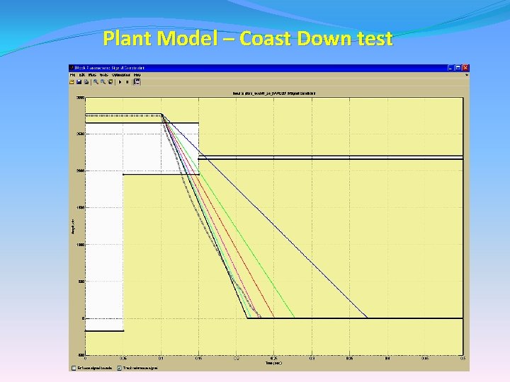
Plant Model – Coast Down test • In vehicle design, a data point for verifying the accuracy of the mechanical model of the vehicle is a coast-down test • Set the engine and motors to zero torque and set the vehicle initial speed and put it to coasts down to zero speed • Tests and measures aerodynamic drag and vehicle frictional losses

Plant Model – Coast Down test • Our goal is found the pressure value of the friction clutch to match the measured coast-down time to the simulated coast-down time • Instead of searching for the clutch pressure manually, we will use the Simulink Response Optimization toolbox • Suppose that we already have a set points from the measured rpm trace

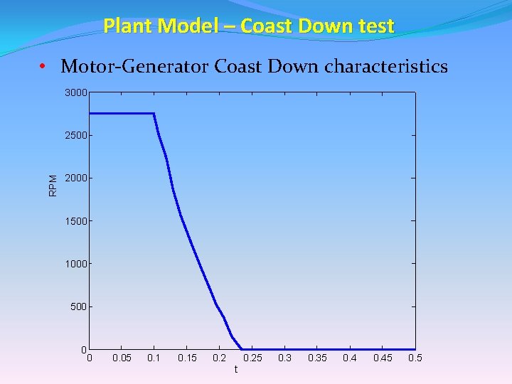
Plant Model – Coast Down test • Motor-Generator Coast Down characteristics 3000 RPM 2500 2000 1500 1000 500 0 0 0. 05 0. 15 0. 2 t 0. 25 0. 35 0. 45 0. 5

Plant Model – Coast Down test • Inside the plant, we need to set the initial condition of speed • We will add a new torque source that balances the torque due to friction • While the forces are balanced, the motor – generator system will maintain the initial rpm, whatever it is • When we want the system to coast-down we set the added torque source to zero

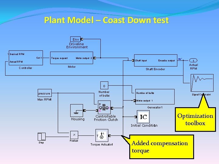
Plant Model – Coast Down test Env Driveline Environment Desired RPM Out 1 Torque request Motor output 2 Motor Controller Encoder output Shaft input Actual RPM 1 Actual RPM Shaft Encoder 0 Number of bulbs pressure Max RPM 1 Number of bulbs Signal Constraint Motor output 1 P B Housing F Generator 1 Controllable Friction Clutch Initial Condition 1 Optimization toolbox T Step Product Torque Actuator 1 Added compensation torque

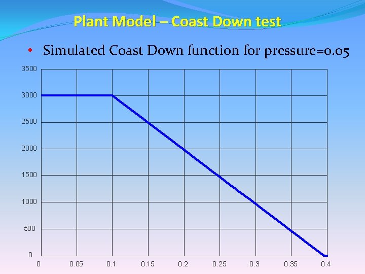
Plant Model – Coast Down test • Simulated Coast Down function for pressure=0. 05 3500 3000 2500 2000 1500 1000 500 0 0 0. 05 0. 15 0. 25 0. 35 0. 4

Plant Model – Coast Down test • We will now use the Math. Works Simulink Response Optimization toolbox to determine the optimum value of the Pressure so that the response of our model matches the measured response • Finally we have results for optimal value of pressure, pressure=1. 1989

Plant Model – Coast Down test • We will now use the Math. Works Simulink Response Optimization toolbox to determine the optimum value of the pressure so that the response of our model matches the measured response • Finally we have results for optimal value of pressure, pressure=1. 1989

Plant Model – Coast Down test

Model Building with Simulink – Friction Model Notes • The proposed friction model has a linear change from high rpm to zero. The actual response looks like an exponential decay – somewhat • Our model of a constant frictional torque is probably too simple • Friction is probably a function of rotational speed and have nonlinear characteristics? ? ?

Model Building with Simulink – Signal Filtering and scaling for ds. PIC ECU • We now need to clean up our model in terms of the signals being sent to the controller • Tacho signal (0 -10 V) is passed through a combination resistive divider and low pass filter to: • Eliminate noise on the signal • Change range to 0 -5 V

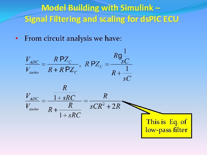
Model Building with Simulink – Signal Filtering and scaling for ds. PIC ECU • From circuit analysis we have: This is Eq. of low-pass filter

Model Building with Simulink – Signal Filtering • Implementation low pass filter in SIMULINK: 10000 1 /5 1 10 s + 20000 Step Low pass filter Scaling gain 1 Saturation 1 Out 2

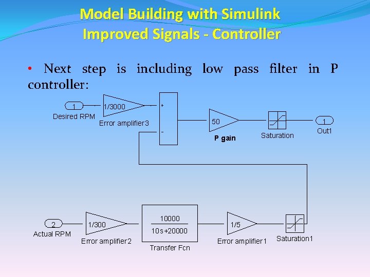
Model Building with Simulink Improved Signals - Controller • Next step is including low pass filter in P controller: 1 Desired RPM 1/3000 50 Error amplifier 3 P gain 2 Actual RPM 1/300 Error amplifier 2 10000 10 s+20000 Transfer Fcn Saturation 1/5 Error amplifier 1 Saturation 1 1 Out 1

Model Building with Simulink Improved Controller - PI • PI Control: • One of our goals is to design a controller for our system • Now that we have a good plant model, we can use all of our knowledge of control systems to design controllers. • We will improve existing controller adding an integrator to our system because: A proportional gain controller yields an error that is inversely proportional to the gain • Too high of a proportional gain can make the system oscillate •

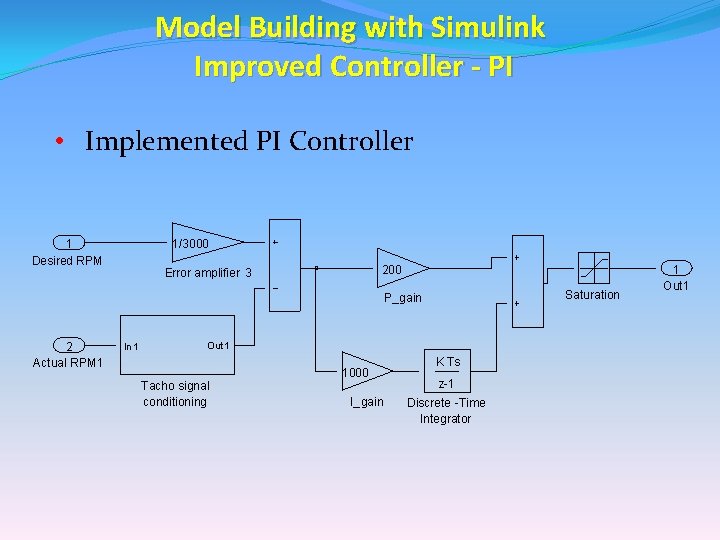
Model Building with Simulink Improved Controller - PI • Implemented PI Controller 1 Desired RPM 1/3000 200 Error amplifier 3 Saturation P_gain 2 Actual RPM 1 In 1 Out 1 Tacho signal conditioning 1000 I_gain K Ts z-1 Discrete -Time Integrator 1 Out 1

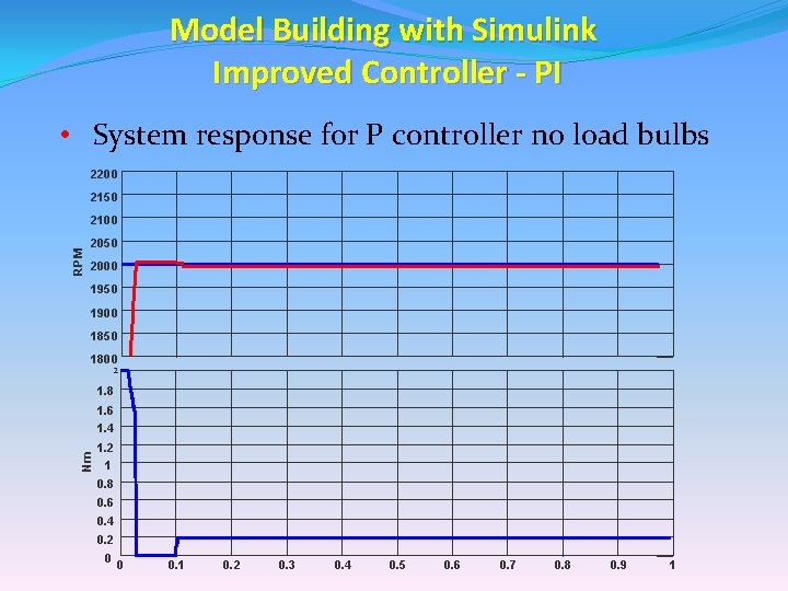
Model Building with Simulink Improved Controller - PI • System response for P controller no load bulbs 2200 2150 RPM 2100 2050 2000 1950 1900 1850 1800 2 1. 8 1. 6 Nm 1. 4 1. 2 1 0. 8 0. 6 0. 4 0. 2 0 0 0. 1 0. 2 0. 3 0. 4 0. 5 0. 6 0. 7 0. 8 0. 9 1

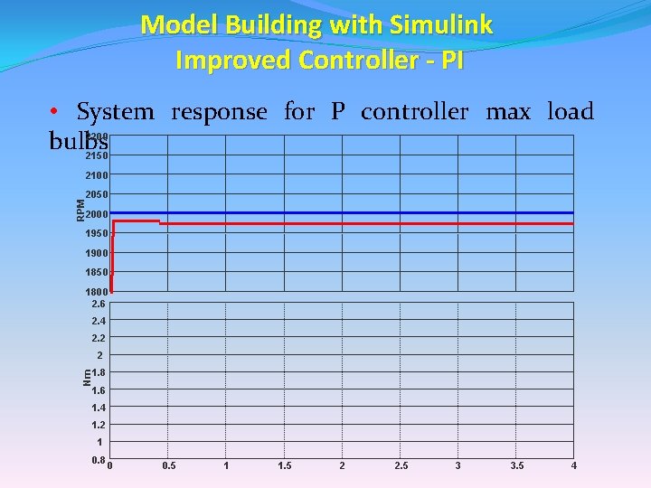
Model Building with Simulink Improved Controller - PI • System response for P controller max load 2200 bulbs 2150 2100 RPM 2050 2000 1950 1900 1850 1800 2. 6 2. 4 2. 2 2 Nm 1. 8 1. 6 1. 4 1. 2 1 0. 8 0 0. 5 1 1. 5 2 2. 5 3 3. 5 4

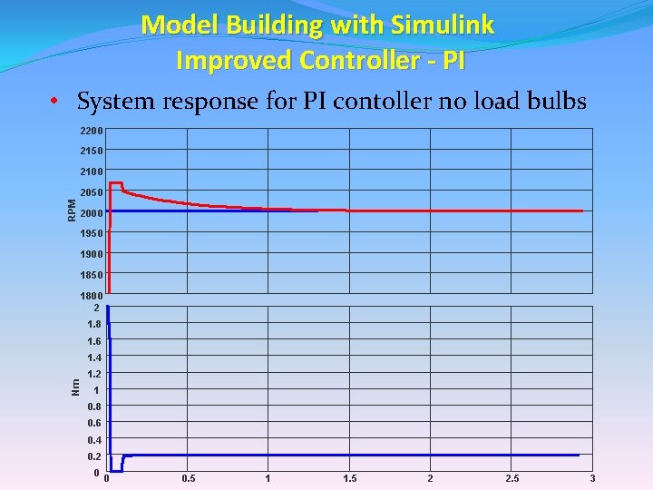
Model Building with Simulink Improved Controller - PI • System response for PI contoller no load bulbs 2200 2150 2100 RPM 2050 2000 1950 1900 1850 1800 2 1. 8 1. 6 Nm 1. 4 1. 2 1 0. 8 0. 6 0. 4 0. 2 0 0 0. 5 1 1. 5 2 2. 5 3

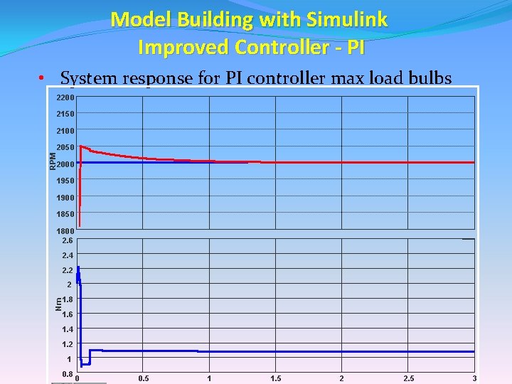
Model Building with Simulink Improved Controller - PI • System response for PI controller max load bulbs 2200 2150 2100 RPM 2050 2000 1950 1900 1850 1800 2. 6 2. 4 2. 2 2 Nm 1. 8 1. 6 1. 4 1. 2 1 0. 8 0 0. 5 1 1. 5 2 2. 5 3

Model Building with Simulink conclusion • MBSD is a powerful technique for complex system design • MBSD can include a lot of different types of models in whole design • MBSD is common part of rapid prototyping process with no waste of time. • We can “Smoke-free" testing all the plant parts

Thank you for attention