Model specification identification We already know about the
 We already know about the sample autocorrelation function (SAC): Properties: •")
Model specification (identification) We already know about the sample autocorrelation function (SAC): Properties: • Not unbiased (since a ratio between two random variables) • Bias decreases with n • Variance complicated, common to use general large-sample results
: For large n the random vector has an approximate multivariate normal")
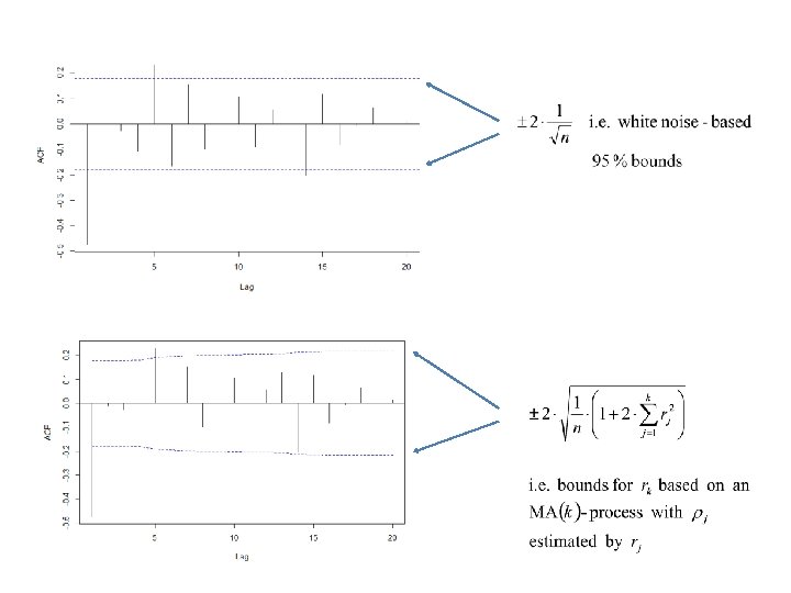
Large-sample results (asymptotics): For large n the random vector has an approximate multivariate normal distribution with zero mean vector and covariance matrix ( cij ) where This gives that Var (rk) 0 as n does not diminish as n

Hence, the distribution of rk will depend on the correlation structure of Yt and accordingly on the model behind (i. e. if it is and AR(1), an ARMA(2, 1) etc. ) For an AR(1), i. e. Yt = Yt – 1 + et i. e. not dependent on k for large lags For an MA(q) i. e. not dependent on k after the qth lag For white noise

Partial autocorrelation function Describes the “specific” part of the correlation between Yt and Yt – k that is not due to successive serial correlations between the variables Yt – 1 , Yt – 2 , …, Yt – k. Partial correlations are used for other types of data as well (for instance in linear models of cross-sectional data. Patterns • For an AR(p)-process, k cuts off after lag p (i. e. the same type of behaviour like k has for an MA(q)-process • For an MA(q)-process k shows approximately the same pattern as does k for an AR(p)-process
: No explicit formula, estimation has")
Estimation from data , Sample Partial Autocorrelation function (SPAC): No explicit formula, estimation has to be made recursively Properties of SPAC: More involved, but for an AR(p)-process SPAC-values for lags greater than p are approximately normally distributed with zero mean and variance 1/n
 One (of several) tool to improve the choice of orders")
Extended Autocorrelation function (EACF) One (of several) tool to improve the choice of orders of ARMA(p, q)-processes. Very clear as a theoretical function, but noisy when estimated on series not too long. AR, MA or ARMA?

No pattern at all?

EACF table for Y AR/MA 0 1 2 3 4 5 6 7 8 9 10 11 12 13 0 oooooo o 1 oooooo o 2 xooooo o o o 3 ooxoooo o o o 4 xooooo o o o 5 xxooooo o 6 oxooooo o 7 oooooxooooo o True process: Yt = 1. 3 + 0. 2 Yt – 1 + et – 0. 1 et – 1 ARMA(0, 0) or ARMA(1, 0)?

Model selection from more analytical tools Dickey-Fuller Unit-Root test H 0: The process Yt is difference non-stationary ( Yt is stationary) Ha : The process Yt is stationary Augmented Dickey-Fuller test statistic (ADF): If =1 (difference non-stationary)
 vs. Ha")
Fit the model and test H 0: a = 0 (difference non-stationary) vs. Ha : a < 0 (stationary) using the test statistic However, not t-distributed under H 0. Another sampling distributions has been derived and tables (programmed in R)
-process, let k = p + q + 1")
Akaike’s criteria For an ARMA(p, q)-process, let k = p + q + 1 and find the values of the parameters p, q, 1 , …, p , 1 , …, q of the model that minimizes • – 2 log{max L(p, q, 1 , …, p , 1 , …, q )} + 2 k AIC [Akaike’s Information Criterion]. Works well when the true process have (at least one) infinite order • – 2 log{max L(p, q, 1 , …, p , 1 , …, q )} + k log(n) BIC [(Schwarz) Bayesian Information Criterion]. Works well when we “know” that the true process is a finite-order ARMA(p, q)
- Slides: 12