Model predictive control and selflearning of thermal models

Model predictive control and selflearning of thermal models for multi-core platforms* Luca Benini Luca. benini@unibo. it *Work supported by Intel Labs Braunschweig

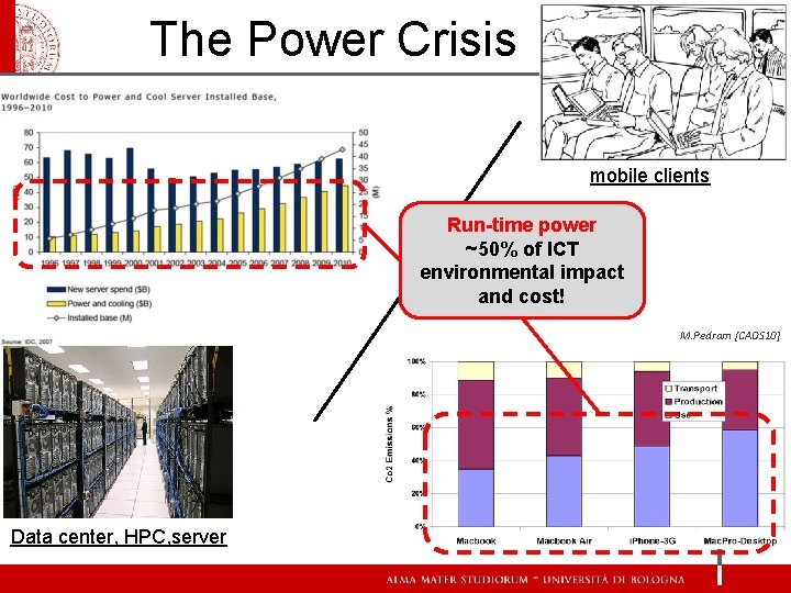
The Power Crisis mobile clients Run-time power ~50% of ICT environmental impact and cost! M. Pedram [CADS 10] Data center, HPC, server

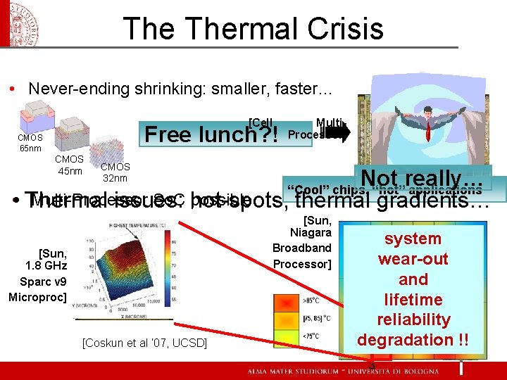
The Thermal Crisis • Never-ending shrinking: smaller, faster… [Cell Free lunch? ! CMOS 65 nm CMOS 45 nm CMOS 32 nm Multi. Processor] Not really… • • Thermal Multi-Processor So. C hot-spots, possible issues: thermal gradients… “Cool” chips, “hot” applications [Sun, Niagara Broadband Processor] [Sun, 1. 8 GHz Sparc v 9 Microproc] [Coskun et al ‘ 07, UCSD] system wear-out and lifetime reliability degradation !! 3

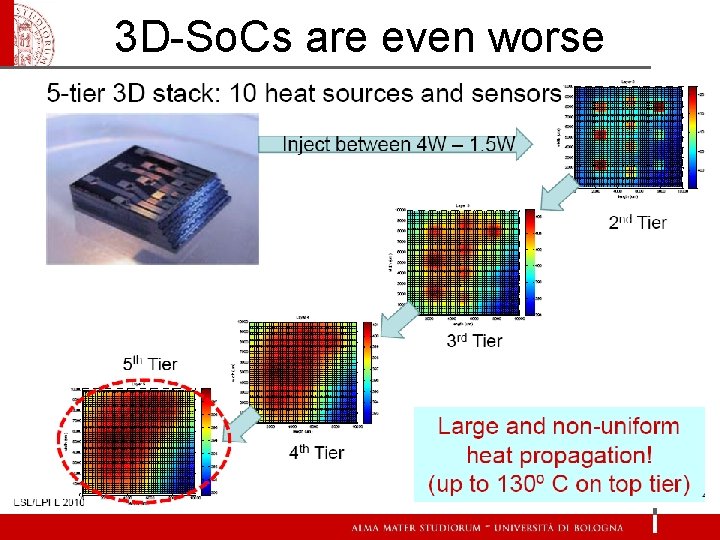
3 D-So. Cs are even worse

A System-level View • Heat density trend 2005 -2010 (systems) [Uptime Institute] Cooling and hot spot avoidance is an open issue!

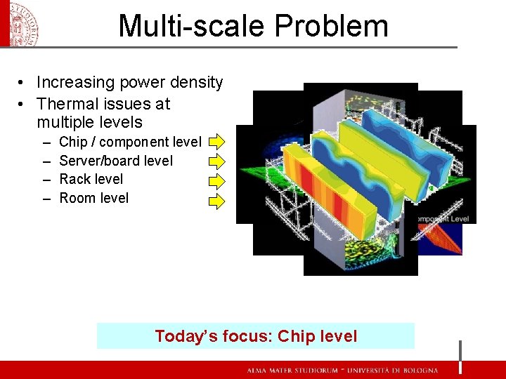
Multi-scale Problem • Increasing power density • Thermal issues at multiple levels – – Chip / component level Server/board level Rack level Room level Today’s focus: Chip level

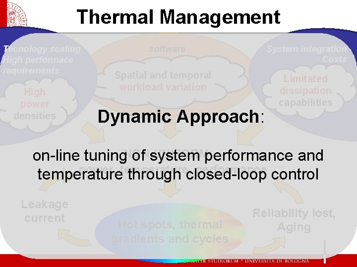
Thermal Management Tecnology scaling High performace requirements High power densities software System integration Costs Spatial and temporal workload variation Dynamic Approach: Limitated dissipation capabilities UNIFORM: on-line tuning. NON of system performance and power, temperature, performance temperature through closed-loop control Leakage current Hot spots, thermal gradients and cycles Reliability lost, Aging

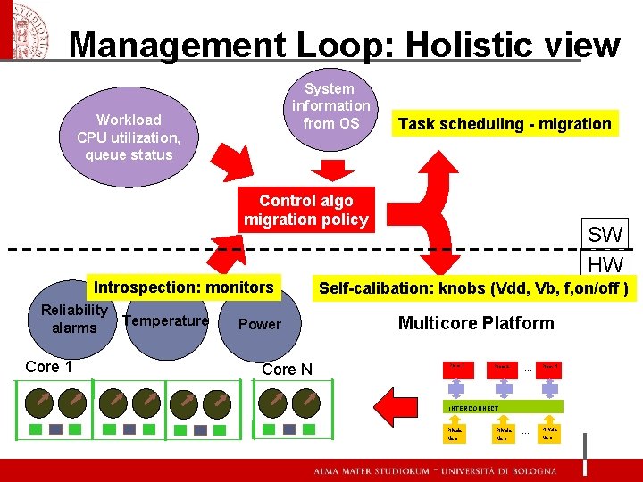
Management Loop: Holistic view System information from OS Workload CPU utilization, queue status Task scheduling - migration Control algo migration policy Introspection: monitors Reliability alarms Core 1 Temperature Power Core N SW HW Self-calibation: knobs (Vdd, Vb, f, on/off ) Multicore Platform Proc. 1 Proc. 2 … Proc. N INTERCONNECT Private Mem … Private Mem

Outline • • Introduction Energy Controller Thermal Controller architecture Learning (self-calibration) Scalability Simulation Infrastructure Results Conclusion

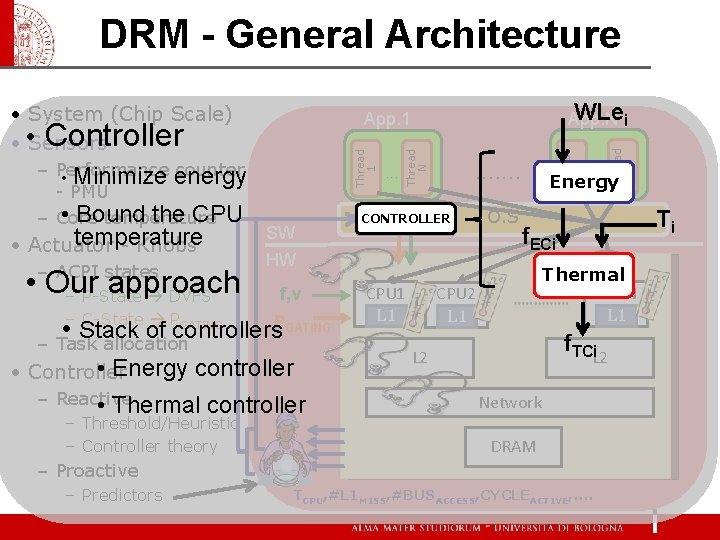
DRM - General Architecture temperature • Actuator - Knobs – ACPI states • Our approach – P-State DVFS SW f, v GATING • Energy controller • Controller controller – Threshold/Heuristic – Controller theory CONTROLLER CPU 1 L 1 Thread 1 . . . . HW – C-State P • Stack of controllers. PGATING – Task allocation – Reactive • Thermal . . . Thread N Thread 1 – Performance counter • Minimize energy - PMU • Bound the CPU – Core temperature WLei App. N App. 1 O. S . . . Energy Ti f. ECi Thermal CPUN L 1 CPU 2 L 1 f. TCi. L 2 Network Simulation snap-shot DRAM – Proactive – Predictors Thread N • System (Chip Scale) Controller • • Sensors TCPU, #L 1 MISS, #BUSACCESS, CYCLEACTIVE, . .

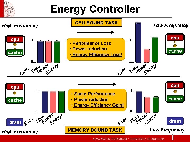
Energy Controller High Frequency cpu 1 CPU BOUND TASK Low Frequency • Performance Loss • Power reduction • Energy Efficiency Loss! cache 0 r gy e e c im ow ner e T P E Ex cpu 1 cache 1 • Same Performance • Power reduction • Energy Efficiency Gain! cache 0 ec dram Ex e wer rgy m Ti Po Ene High Frequency 0 Ex MEMORY BOUND TASK ec e wer rgy m Ti Po Ene dram Low Frequency

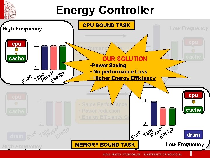
Energy Controller High Frequency cpu 1 CPU BOUND TASK Low Frequency cpu 1 cache 0 r gy e e c im ow ner e T P E Ex • Performance Loss • Power reduction OUR SOLUTION • Energy Efficiency Loss! • Power Saving 0 • No performance Loss r gy e e c im ow ner • Higher Energy Efficiency e T P E Ex cache cpu 1 cache 1 • Same Performance • Power reduction • Energy Efficiency Gain! cache 0 ec dram Ex e wer rgy m Ti Po Ene High Frequency 0 Ex MEMORY BOUND TASK ec e wer rgy m Ti Po Ene dram Low Frequency

Outline • • Introduction Energy Controller Thermal Controller architecture Learning (self-calibration) Scalability Simulation Infrastructure Results Conclusion

Thermal Controller E L P M [Intel®, ISSCC 2007] Y T I X CO Classical feed-back controller Threshold based controller • T > Tmax low freq • T < Tmin high freq • cannot prevent overshoot • thermal cycle • PID controllers • Better than threshold based approach • Cannot prevent overshoot Model Predictive Controller • Internal prediction: avoid overshoot • Optimization: maximizes performance Target frequency Past input & output Thermal Model Future output - + Future Optimizer error input Cost function Constraint MPC • Centralized • aware of neighbor cores thermal influence • All at once – MIMO controller • Complexity !!!

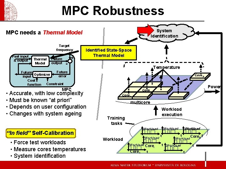
MPC Robustness System Identification MPC needs a Thermal Model Target frequency Past input & output Thermal Model Future output - + Identified State-Space Thermal Model Temperature Future Optimizer error input Cost function Constraint Core. N MPC • Accurate, with low complexity • Must be known “at priori” • Depends on user configuration • Changes with system ageing Core 1 multicore Workload execution Training tasks Workload “In field” Self-Calibration • Force test workloads • Measure cores temperatures • System identification Power Corei Workload Core i Core 1 t t Workload t Core. N t Workload t t

Outline • • Introduction Energy Controller Thermal Controller architecture Learning (self-calibration) Scalability Simulation Infrastructure Results Conclusion

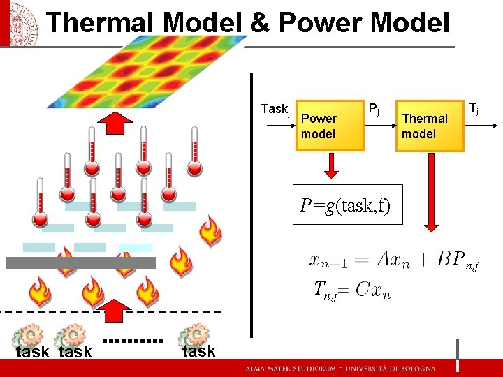
Thermal Model & Power Model Taskj Power di Modello potenza model Pj Thermal Modello Termico model Tj P=g(task, f) Pn, j Tn, j task

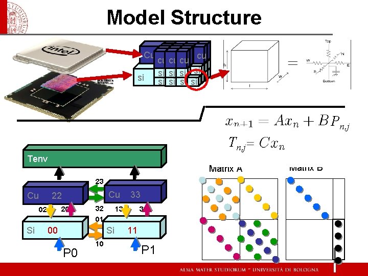
Model Structure Cu si cu cu si si Pn, j Tenv Matrix A 23 Cu 20 02 Si Cu 22 32 01 13 Si 00 P 0 10 33 31 11 P 1 Matrix B

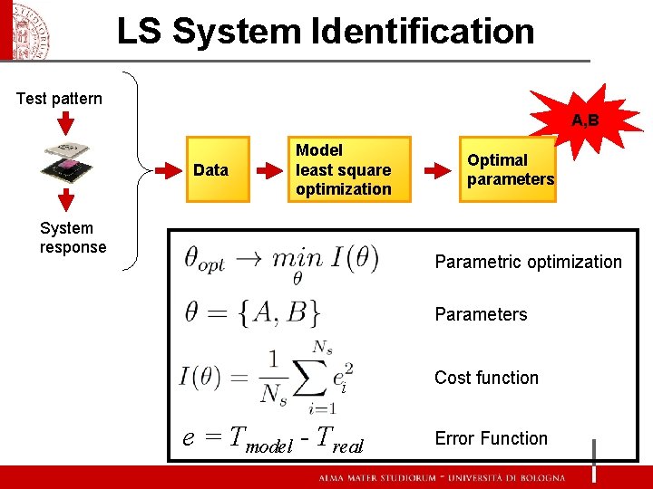
LS System Identification Test pattern A, B Data Model least square optimization System response Optimal parameters Parametric optimization Parameters i e = Tmodel - Treal Cost function Error Function

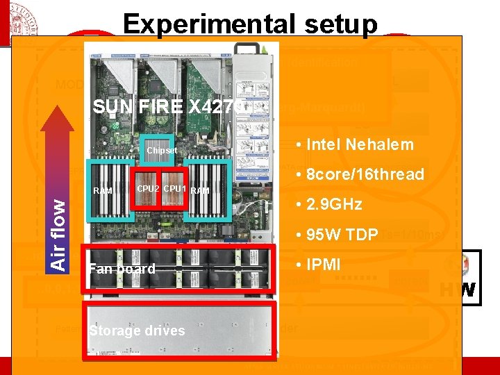
Experimental setup MODEL SUN LS Matlab System Identification C/FORTRAN • N 4 SID MODEL (SLICOT, MINPACK) • PEM • LS (Levenberg-Marquardt) FIRE X 4270 LS • Intel Nehalem Chipset DATA. csv Air flow CPU 2 CPU 1 RAM • Temperature • Frequency • Workload RAM • 2. 9 GHz XTS . . idle, run, … Fan board . . 0, 0, 1, 1, 1, … PRBS. csv Storage drives Pattern Generator PREPROCESSING • 8 core/16 thread PREPROCESSING • 95 W TDP(Ts=1/10 ms) • IPMI core 0 core 1 Workloader core. N HW

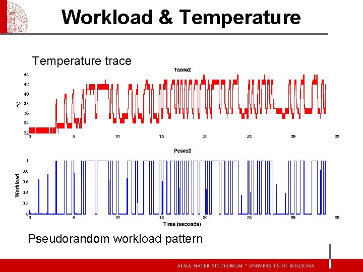
Workload & Temperature trace Pseudorandom workload pattern

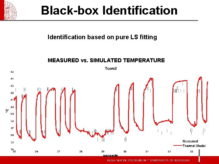
Black-box Identification based on pure LS fitting MEASURED vs. SIMULATED TEMPERATURE TEMPERATURA MISURATA vs. SIMULATA

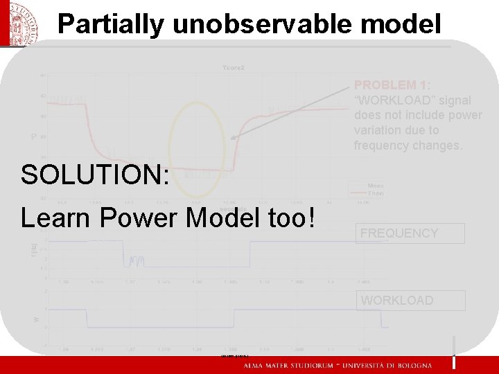
Partially unobservable model PROBLEM 1: “WORKLOAD” signal does not include power variation due to frequency changes. SOLUTION: Learn Power Model too! FREQUENCY WORKLOAD

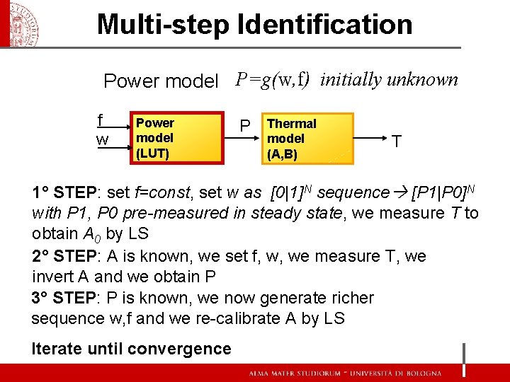
Multi-step Identification Power model P=g(w, f) initially unknown f w Power model (LUT) P Thermal model (A, B) T 1° STEP: set f=const, set w as [0|1]N sequence [P 1|P 0]N with P 1, P 0 pre-measured in steady state, we measure T to obtain A 0 by LS 2° STEP: A is known, we set f, w, we measure T, we invert A and we obtain P 3° STEP: P is known, we now generate richer sequence w, f and we re-calibrate A by LS Iterate until convergence

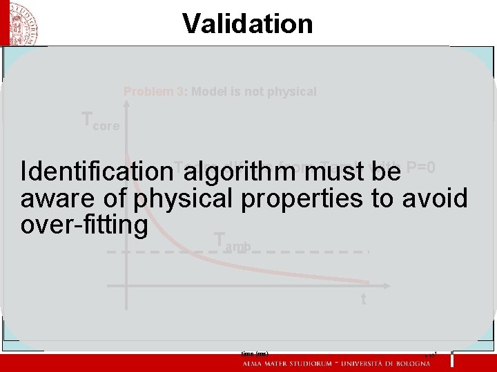
Validation Problem 3: Model is not physical Problem 2: Instable Model Tcore differs from Tamb with Identification. Tcore algorithm must be P=0 aware of physical properties to avoid over-fitting T amb t

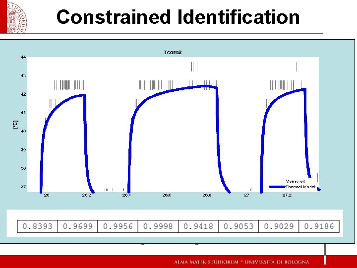
Constrained Identification Constraint on initial condition Linear constraint CONSTRAINED LEAST SQUARES

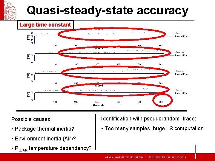
Quasi-steady-state accuracy Large time constant Possible causes: Identification with pseudorandom trace: • Package thermal inertia? • Too many samples, huge LS computation • Environment inertia (Air)? • PLEAK temperature dependency?

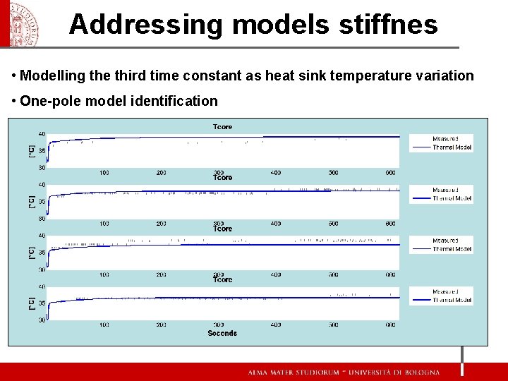
Addressing models stiffnes • Modelling the third time constant as heat sink temperature variation • One-pole model identification Tenv Enviroment thermal model Theatsink T CPU thermal model P

Outline • • Introduction Energy Controller Thermal Controller architecture Learning (self-calibration) Scalability Simulation Infrastructure Results Conclusion

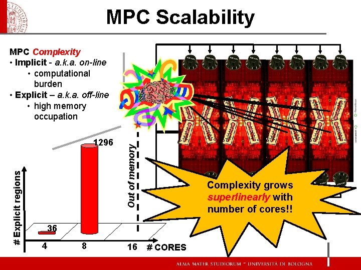
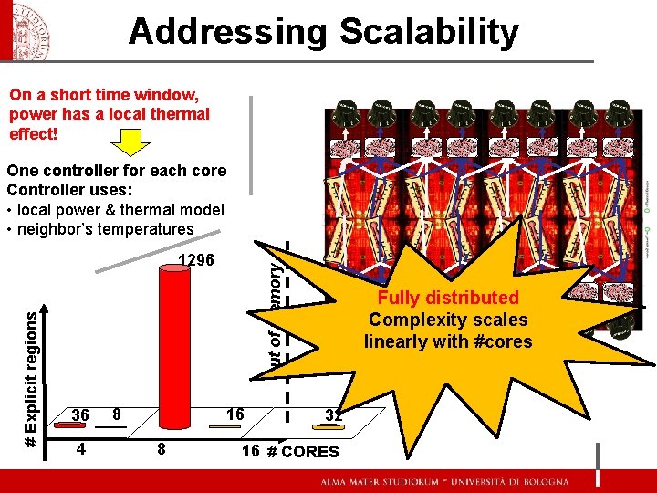
MPC Scalability MPC Complexity • Implicit - a. k. a. on-line • computational burden • Explicit – a. k. a. off-line • high memory occupation # Explicit regions 1296 Out of memory [Intel, ISSCC 2007] 8 16 [Intel, ISSCC 2007] Complexity grows superlinearly with number of cores!! 36 4 [Intel, ISSCC 2007] # CORES [Intel, ISSCC 2007]

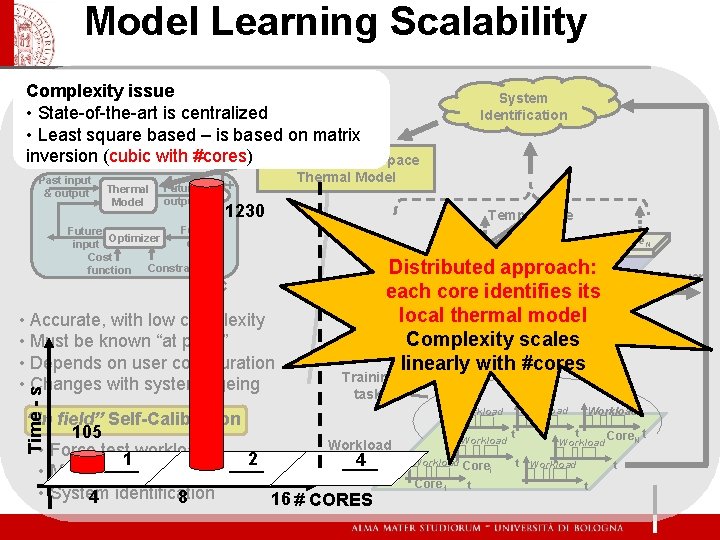
Addressing Scalability On a short time window, power has a local thermal effect! One controller for each core Controller uses: • local power & thermal model • neighbor’s temperatures 36 4 8 Out of memory # Explicit regions 1296 16 8 Fully distributed Complexity scales linearly with #cores 32 16 # CORES

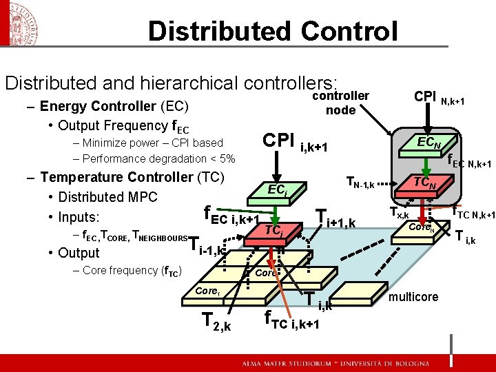
Distributed Control Distributed and hierarchical controllers: controller node – Energy Controller (EC) • Output Frequency f. EC – Minimize power – CPI based – Performance degradation < 5% CPI i, k+1 – Temperature Controller (TC) ECi • Distributed MPC f. EC i, k+1 • Inputs: – f. EC , TCORE, TNEIGHBOURS • Output Ti-1, k – Core frequency (f. TC) CPI N, k+1 TCi ECN f. EC N, k+1 TN-1, k Ti+1, k TCN Tx, k Core. N Corei Core 1 T 2, k T i, k f. TC i, k+1 multicore f. TC N, k+1 T i, k

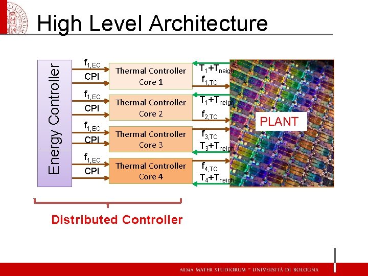
Energy Controller High Level Architecture f 1, EC CPI Thermal Controller Core 1 T 1+Tneigh f 1, TC Thermal Controller Core 2 T 1+Tneigh Thermal Controller Core 3 f 3, TC T 3+Tneigh Thermal Controller Core 4 f 4, TC T 4+Tneigh Distributed Controller f 2, TC PLANT

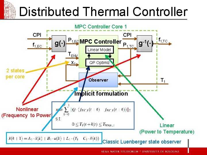
Distributed Thermal Controller MPC Controller Core 1 CPI f 1, EC g(·) P 1, EC MPC Controller TENV x 1 2 states per core Linear Model CPI P 1, TC g-1(·) f 1, TC QP Optimiz Observer T 1 Implicit formulation Nonlinear (Frequency to Power) s. t Linear (Power to Temperature) Classic Luenberger state observer

Explicit Distributed Controller x 1 [x 1 ; TENV ; P 1, EC] A 1 -1·B 1 + x 1 SHIFTED ? Region number REGION GAIN NUMBER MATRICES 1 F 1 , G 1 2 … F 2 , G 2 … nr Fnr , Gnr u(k)=∆P 1 + P 1, TC P 1, EC The prediction evaluated by our explicit controller cannot take into account the Our aim is to minimize the difference between the input P 1, TC (also called measured disturbances (u. MD=[Tenv, P 1, ]). Thus we exploit the superposition Atthe each time. Tneigh instant system belongs to atake region manipulated variable MV) and reference (P 1, EC). the Our controller can only in principle of linear systems: according with its current state. On each region the account a constant reference. To overcome this limitation we reformulate the explicit controller executes following control tracking problem as a regulation problem consisting in the taking the ∆Plinear 1 (the new To remap theregulated effect of power theselaw: elements MV) to 0. The P 1, TC is: we exploit the model to modify the state (x(k) x. SHIFTED(k)) projecting one step forward the MDs effects.

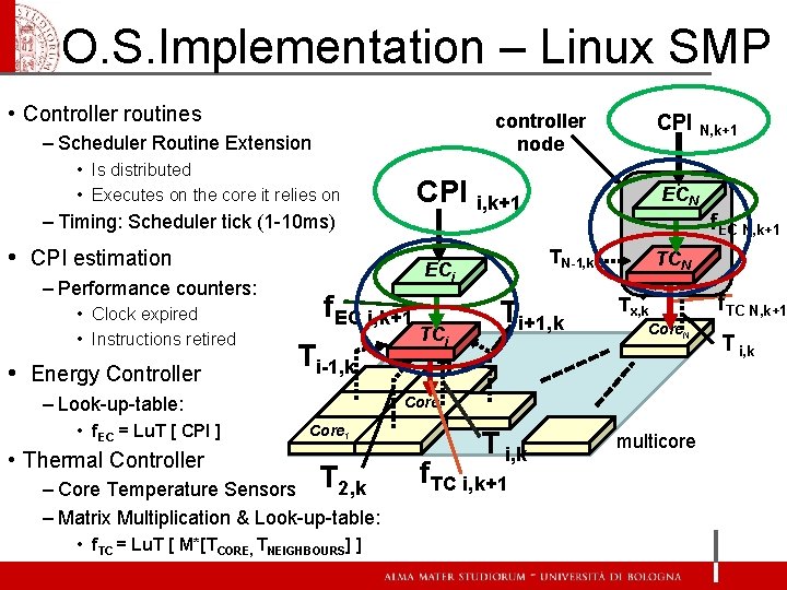
O. S. Implementation – Linux SMP • Controller routines controller node – Scheduler Routine Extension • Is distributed • Executes on the core it relies on CPI i, k+1 – Timing: Scheduler tick (1 -10 ms) • CPI estimation – Performance counters: • Clock expired • Instructions retired • Energy Controller f. EC i, k+1 – Look-up-table: • f. EC = Lu. T [ CPI ] TCi ECN f. EC N, k+1 TN-1, k ECi Ti-1, k CPI N, k+1 Ti+1, k TCN Tx, k Core. N Corei Core 1 • Thermal Controller – Core Temperature Sensors T 2, k – Matrix Multiplication & Look-up-table: • f. TC = Lu. T [ M*[TCORE, TNEIGHBOURS] ] T i, k f. TC i, k+1 multicore f. TC N, k+1 T i, k

Model Learning Scalability Complexity issue MPC Weaknesses – 2 nd • State-of-the-art is centralized Internal Thermal Model • Least square based – is based on matrix Target inversion (cubic withfrequency #cores) Identified State-Space Past input & output Thermal Model Future output + Thermal Model - 1230 Future Optimizer error input Cost function Constraint MPC • Accurate, with low complexity • Must be known “at priori” • Depends on user configuration • Changes with system ageing Time - s System Identification Temperature >1 h Core. N Distributed approach: Core each core identifies its Core local thermal model multicore Complexity Workload scales linearly withexecution #cores Power i 1 Training tasks “In field” Self-Calibration 105 Workload • Force test workloads 1 2 4 • Measure cores temperatures • System 4 identification 8 16 # CORES Workload Core i Core 1 t t Workload t Core. N t Workload t t

Outline • • Introduction Energy Controller Thermal Controller architecture Learning (self-calibration) Scalability Simulation Infrastructure Results Conclusion

Simulation Strategy Trace driven Simulator [1]: • • Not suitable for full system simulation (How to simulate O. S. ? ) looses information on cross-dependencies resulting in degraded simulation accuracy Close loop simulator: Cycle accurate simulators [2] : • • • High modeling accuracy support well-established power and temperature co-simulation based on analytical models and system micro-architectural knowledge Low simulation speed Not suitable for full-system simulation Functional and instruction set simulators: • • allow full system simulation less internal precision less detailed data no micro-architectural model introduces the challenge of having accurate power and temperature physical models Control strategy • Workload Set Workload Multicore Simulator Execution Trace database Power Model Temperature Model [1] P Chaparro et al. Understanding thermal implications of multi-core architectures. 2007 [2] Benini L. et al. MPARM: Exploring the multi-processor So. C design space with System. C 2005

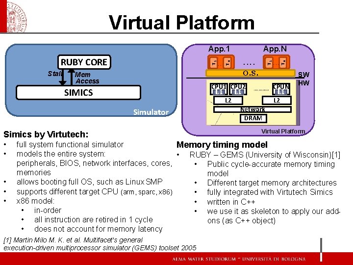
Virtual Platform Stall Simulator Simics by Virtutech: • • • T 1 . . . . O. S. Mem Access SIMICS • • . . . TN T 1 RUBY CORE TN App. 1 CPU 2 L 1 L 2 Network DRAM CPUN L 1 L 2 SW HW Virtual Platform full system functional simulator Memory timing models the entire system: • RUBY – GEMS (University of Wisconsin)[1] peripherals, BIOS, network interfaces, cores, • Public cycle-accurate memory timing memories model allows booting full OS, such as Linux SMP • Different target memory architectures supports different target CPU (arm, sparc, x 86) • fully integrated with Virtutech Simics x 86 model: • written in C++ • in-order • we use it as skeleton to apply our add • all instruction are retired in 1 cycle ons (as C++ object) • does not account for memory latency [1] Martin Milo M. K. et al. Multifacet’s general execution-driven multiprocessor simulator (GEMS) toolset 2005

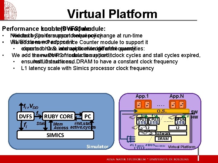
Virtual Platform knobs (DVFS) module: Performance counters module: DVFS fi RUBY CORE Stall PC #hlt, stall Mem active, cycles Access SIMICS Simulator . . . . O. S. f, v CPU 1 CPU 2 L 1 L 2 Network DRAM . . . TN fi , VDD fi T 1 App. N App. 1 TN • Virtutechby. Simics supportcontrol frequency change at run-time Needed performance policy RUBY not. Performance support it: Counter module to support it We adddoes a new does not knowledge of frequency • exports tohave O. S. internal and application different quantities: We add new DVFSofmodule to support : • a the number instruction retired, itclock cycles and stall cycles expired, • ensures cache and DRAM to have a constant clock frequency halt. L 2 instructions, … • L 1 latency scale with Simics processor clock frequency T 1 • • SW f, v HW CPUN L 1 L 2 #L 1 MISS, #BUSACCESS, Virtual Platform CYCLE ACTIVE, . .

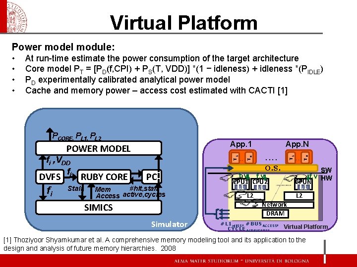
Virtual Platform Power model module: At run-time estimate the power consumption of the target architecture Core model PT = [PD(f, CPI) + PS(T, VDD)] *(1 − idleness) + idleness *(PIDLE) PD experimentally calibrated analytical power model Cache and memory power – access cost estimated with CACTI [1] DVFS fi RUBY CORE Stall PC #hlt, stall Mem active, cycles Access SIMICS Simulator . . . . O. S. f, v CPU 1 CPU 2 L 1 L 2 Network DRAM . . . TN T 1 fi , VDD fi App. N App. 1 POWER MODEL T 1 PCORE, PL 1, PL 2 TN • • SW f, v HW CPUN L 1 L 2 #L 1 MISS, #BUSACCESS, Virtual Platform CYCLE ACTIVE, . . [1] Thoziyoor Shyamkumar et al. A comprehensive memory modeling tool and its application to the design and analysis of future memory hierarchies. 2008

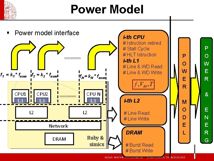
Power Model § Power model interface i-th CPU # Istruction retired # Stall Cycle # HLT Istruction i-th L 1 f 1 = k 1 * fnom f 2 = k 2 * fnom CPU 1 L 1 CPU 2 L 1 f. N = k. N * fnom CPU N L 1 L 2 # Line & WD Read # Line & WD Write & i-th L 2 # Line Read # Line Write Network Simulation snap-shot DRAM Ruby & simics P O W E R DRAM # Burst Read # Burst Write M O D E L E N E R G Y

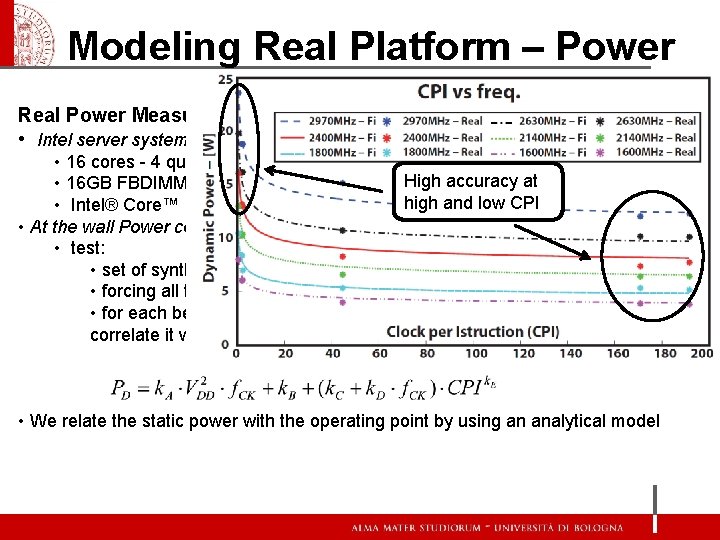
Modeling Real Platform – Power Real Power Measurement • Intel server system S 7000 FC 4 UR • 16 cores - 4 quad cores Intel® Xeon® X 7350, 2. 93 GHz High accuracy at • 16 GB FBDIMMs high and low CPI • Intel® Core™ 2 Duo architecture • At the wall Power consumption • test: • set of synthetic benchmarks with different memory pattern accesses • forcing all the cores to run at different performance levels • for each benchmark we extract the clocks per instruction metrics (CPI) and correlate it with the power consumption • We relate the static power with the operating point by using an analytical model

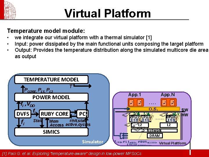
Virtual Platform Temperature model module: • • • we integrate our virtual platform with a thermal simulator [1] Input: power dissipated by the main functional units composing the target platform Output: Provides the temperature distribution along the simulated multicore die area as output TEMPERATURE MODEL T DVFS fi RUBY CORE Stall PC #hlt, stall Mem Access active, cycles SIMICS Simulator . . O. S. f, v CPU 1 CPU 2 L 1 L 2 Network DRAM . . . TN . . . T 1 fi , VDD fi App. N App. 1 POWER MODEL TN PCORE, PL 1, PL 2 SW f, v HW CPUN L 1 L 2 TCPU, #L 1 MISS, #BUSACCESS, Virtual Plattform CYCLE ACTIVE, . . [1] Paci G. et al. Exploring ”temperature-aware” design in low-power MPSo. Cs

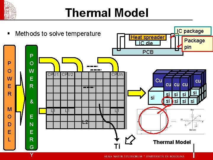
Thermal Model IC package § Methods to solve temperature P O W E R PCB CPU 1 CPU 2 PCPU 1 PL 1 E N E R G Y Package pin CPUn Cu & M O D E L Heat spreader IC die PCPU 2 PL 1 L 2 PCPUn PL 1 L 2 L 1 si cu cu cu si si L 1 Network L 2 Ti cu Thermal Model

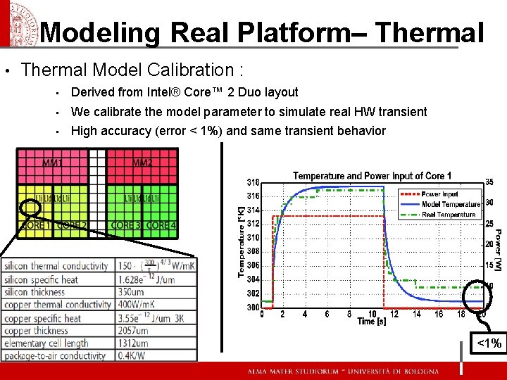
Modeling Real Platform– Thermal • Thermal Model Calibration : • Derived from Intel® Core™ 2 Duo layout • We calibrate the model parameter to simulate real HW transient • High accuracy (error < 1%) and same transient behavior <1%

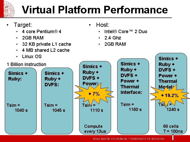
Virtual Platform Performance • Target: • • • Host: 4 core Pentium® 4 2 GB RAM 32 KB private L 1 cache 4 MB shared L 2 cache Linux OS 1 Billion instruction Simics + Ruby: Simics + Ruby + DVFS: • Intel® Core™ 2 Duo • 2. 4 Ghz • 2 GB RAM Simics + Ruby + DVFS + Power: + 7% Tsim = 1040 s Tsim = 1045 s Tsim = 1110 s Compute every 13 us Simics + Ruby + DVFS + Power + Thermal interface: Tsim = 1160 s Simics + Ruby + DVFS + Power + Thermal Model: + 19. 2% Tsim = 1240 s 68 cells T = 100 ns

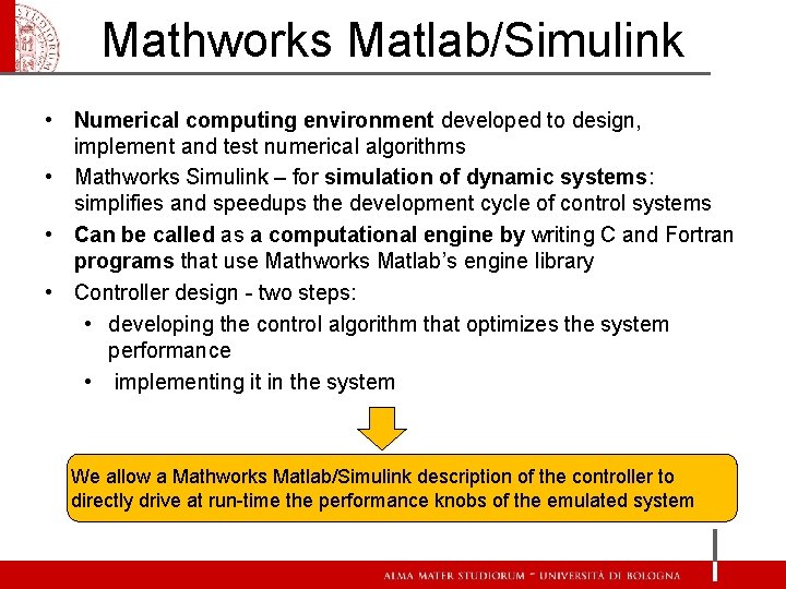
Mathworks Matlab/Simulink • Numerical computing environment developed to design, implement and test numerical algorithms • Mathworks Simulink – for simulation of dynamic systems: simplifies and speedups the development cycle of control systems • Can be called as a computational engine by writing C and Fortran programs that use Mathworks Matlab’s engine library • Controller design - two steps: • developing the control algorithm that optimizes the system performance • implementing it in the system We allow a Mathworks Matlab/Simulink description of the controller to directly drive at run-time the performance knobs of the emulated system

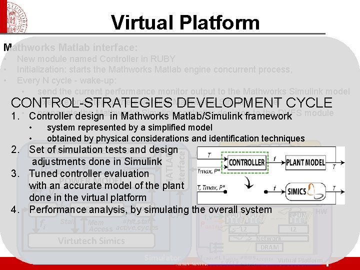
Virtual Platform Mathworks Matlab interface: New module named Controller in RUBY Initialization: starts the Mathworks Matlab engine concurrent process, Every N cycle - wake-up: • send the current performance monitor output to the Mathworks Simulink model • execute one step of the controller Mathworks Simulink model CYCLE CONTROL-STRATEGIES DEVELOPMENT propagatedesign the Mathworks Simulink. Matlab/Simulink controller decision to the DVFS module 1. • Controller in Mathworks framework system represented by a simplified model obtained by physical considerations and identification techniques Mathwor ks Matlab • • TN T 1 TN 2. Set. TEMPERATURE of simulation tests and design MODEL P, T Controller adjustments done in TSimulink PCORE, PL 1, PL 2 P 3. Tuned controller evaluation App. N App. 1 POWER MODEL with an accurate model of the plant. . fi , VDD done in the virtual platform O. S. fi DVFS RUBY CORE by. PC 4. Performance analysis, simulating the overall system CPU 1 CPU 2 CPUN CPI f, v L 1 L 1 Stall #hlt, stall Mem P fi GATING L 2 Access active, cycles MATLAB Interface • • • SW HW Network DRAM Virtutech Simics Simulator TCPU, #L 1 MISS, #BUSACCESS, Virtual Platform CYCLE ACTIVE, . .

Outline • • Introduction Energy Controller Thermal Controller architecture Learning (self-calibration) Scalability Simulation Infrastructure Results Conclusion

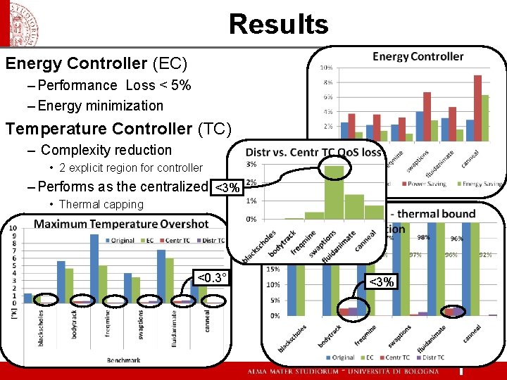
Results Energy Controller (EC) – Performance Loss < 5% – Energy minimization Temperature Controller (TC) – Complexity reduction • 2 explicit region for controller – Performs as the centralized <3% • Thermal capping <0. 3° <3%

Next Steps • Now working on the embedded implementation • Server multicore platform and Intel ® SCC • Explore thermal aware scheduler solution • co-operate with presented solution • Develop distributed+multi-scale solution for data-centers

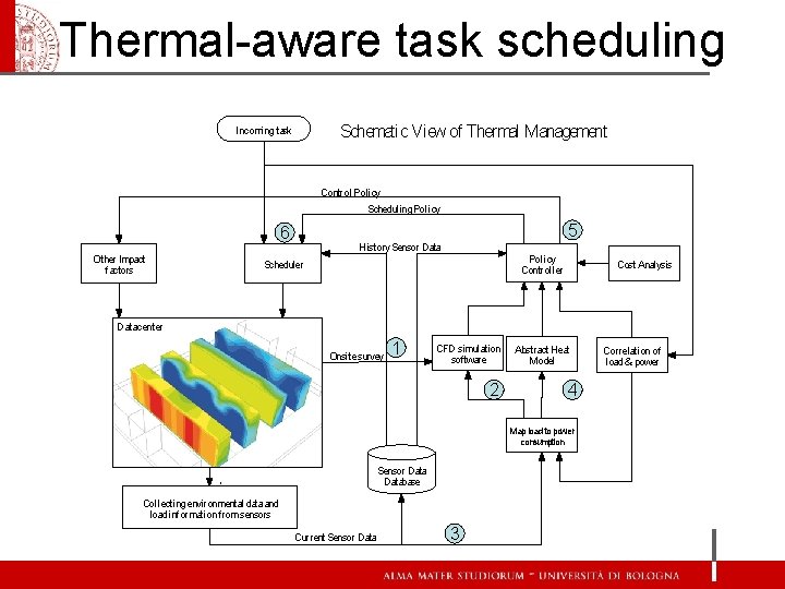
Thermal-aware task scheduling Schematic View of Thermal Management Incoming task Control Policy Scheduling Policy 5 6 Other Impact factors History Sensor Data Policy Controller Scheduler Cost Analysis Datacenter Onsite survey 1 CFD simulation software 2 Abstract Heat Model 4 Map load to power consumption Sensor Database ` Collecting environmental data and load information from sensors Current Sensor Data 3 Correlation of load & power

Thank you!