Model Parts and Structure History of Idea Fischler

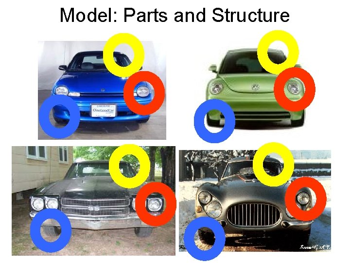
Model: Parts and Structure

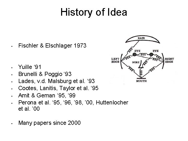
History of Idea • • Fischler & Elschlager 1973 Yuille ‘ 91 Brunelli & Poggio ‘ 93 Lades, v. d. Malsburg et al. ‘ 93 Cootes, Lanitis, Taylor et al. ‘ 95 Amit & Geman ‘ 95, ‘ 99 Perona et al. ‘ 95, ‘ 96, ’ 98, ’ 00, Huttenlocher et al. ’ 00 Many papers since 2000

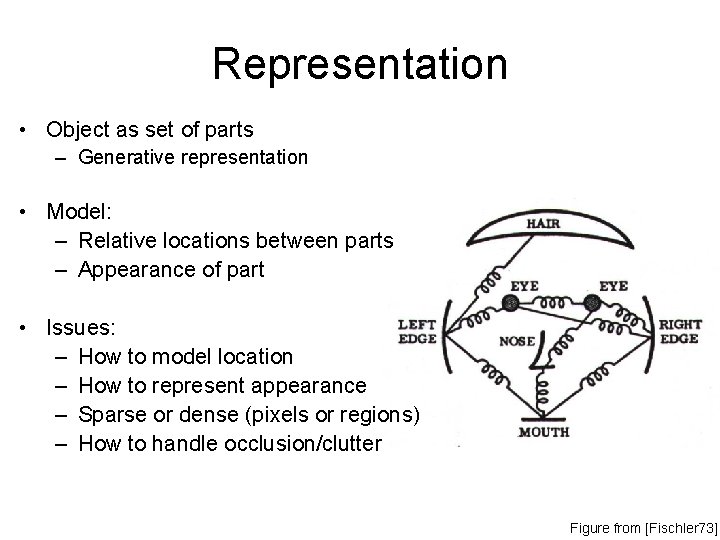
Representation • Object as set of parts – Generative representation • Model: – Relative locations between parts – Appearance of part • Issues: – How to model location – How to represent appearance – Sparse or dense (pixels or regions) – How to handle occlusion/clutter Figure from [Fischler 73]

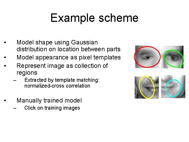
Example scheme • Model shape using Gaussian distribution on location between parts Model appearance as pixel templates Represent image as collection of regions • • – • Extracted by template matching: normalized-cross correlation Manually trained model – Click on training images

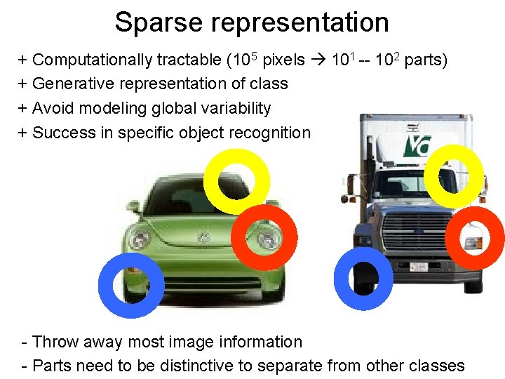
Sparse representation + Computationally tractable (105 pixels 101 -- 102 parts) + Generative representation of class + Avoid modeling global variability + Success in specific object recognition - Throw away most image information - Parts need to be distinctive to separate from other classes

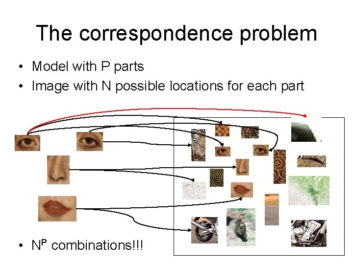
The correspondence problem • Model with P parts • Image with N possible locations for each part • NP combinations!!!

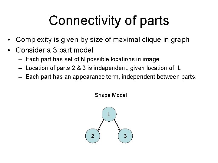
Connectivity of parts • Complexity is given by size of maximal clique in graph • Consider a 3 part model – Each part has set of N possible locations in image – Location of parts 2 & 3 is independent, given location of L – Each part has an appearance term, independent between parts. Shape Model L 2 3

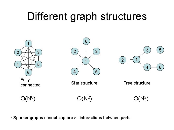
Different graph structures 6 1 2 3 4 2 Fully connected O(N 6) 2 1 5 6 3 4 5 Star structure 3 5 4 6 1 Tree structure O(N 2) • Sparser graphs cannot capture all interactions between parts O(N 2)

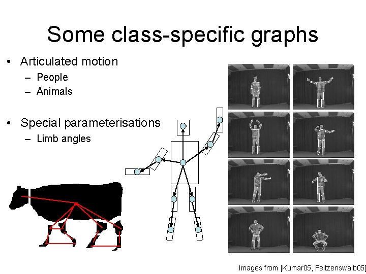
Some class-specific graphs • Articulated motion – People – Animals • Special parameterisations – Limb angles Images from [Kumar 05, Feltzenswalb 05]

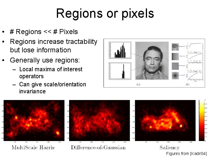
Regions or pixels • # Regions << # Pixels • Regions increase tractability but lose information • Generally use regions: – Local maxima of interest operators – Can give scale/orientation invariance Figures from [Kadir 04]

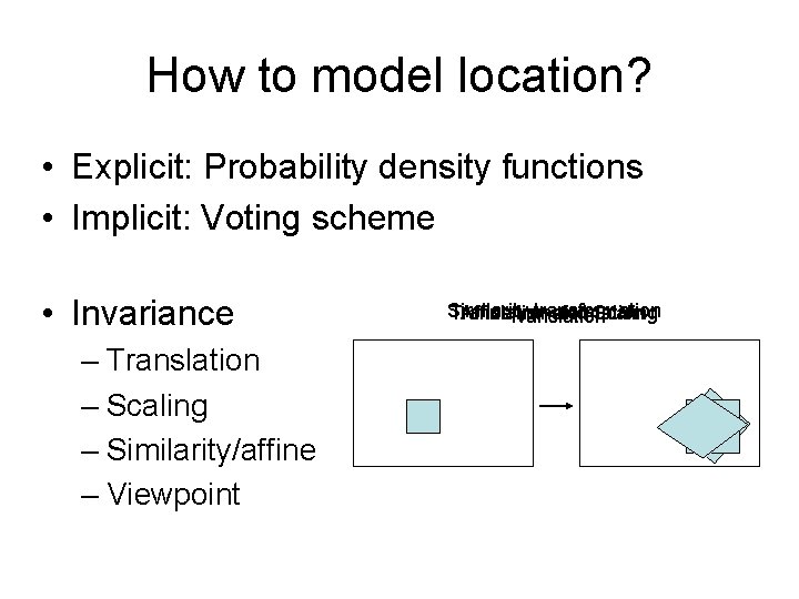
How to model location? • Explicit: Probability density functions • Implicit: Voting scheme • Invariance – Translation – Scaling – Similarity/affine – Viewpoint Similarity transformation Translation Affine. Translation transformation and Scaling

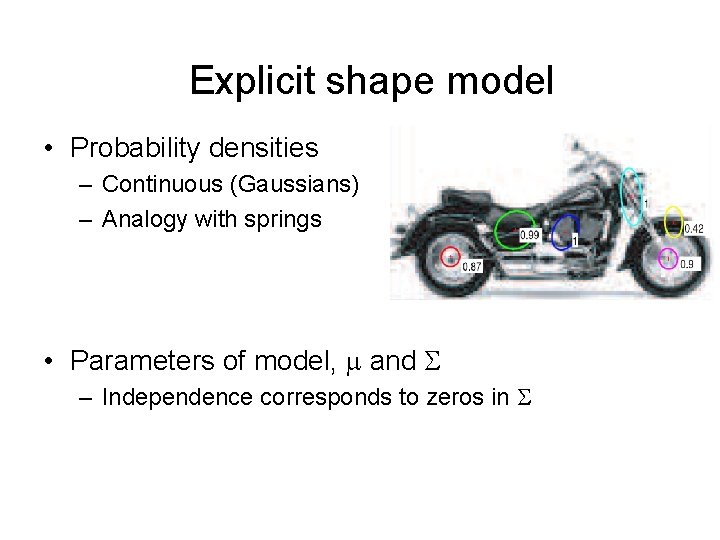
Explicit shape model • Probability densities – Continuous (Gaussians) – Analogy with springs • Parameters of model, and – Independence corresponds to zeros in

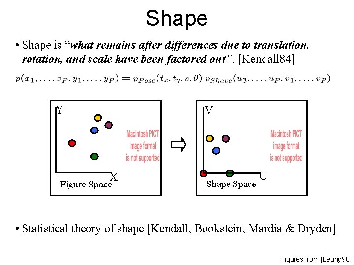
Shape • Shape is “what remains after differences due to translation, rotation, and scale have been factored out”. [Kendall 84] Y V X Figure Space Shape Space U • Statistical theory of shape [Kendall, Bookstein, Mardia & Dryden] Figures from [Leung 98]

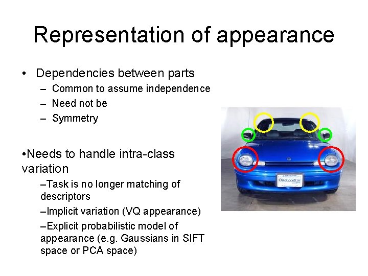
Representation of appearance • Dependencies between parts – Common to assume independence – Need not be – Symmetry • Needs to handle intra-class variation –Task is no longer matching of descriptors –Implicit variation (VQ appearance) –Explicit probabilistic model of appearance (e. g. Gaussians in SIFT space or PCA space)

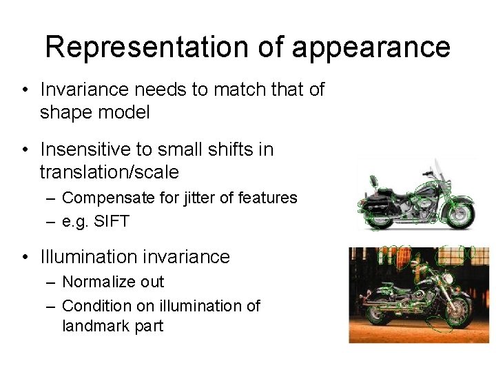
Representation of appearance • Invariance needs to match that of shape model • Insensitive to small shifts in translation/scale – Compensate for jitter of features – e. g. SIFT • Illumination invariance – Normalize out – Condition on illumination of landmark part

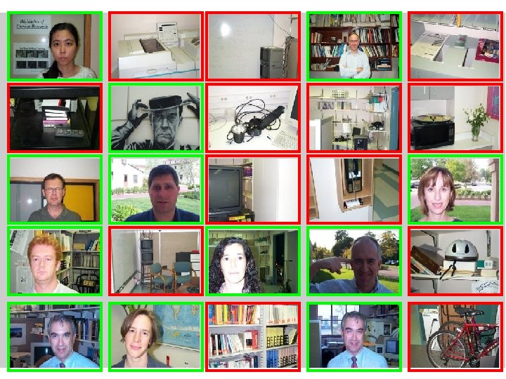
Parts and Structure demo • Gaussian location model – star configuration • Translation invariant only – Use 1 st part as landmark • Appearance model is template matching • Manual training – User identifies correspondence on training images • Recognition – – Run template for each part over image Get local maxima set of possible locations for each part Impose shape model - O(N 2 P) cost Score of each match is combination of shape model and template responses.

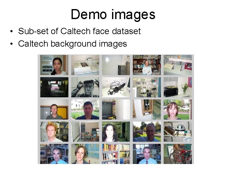
Demo images • Sub-set of Caltech face dataset • Caltech background images

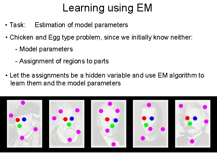
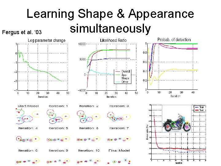
Learning using EM • Task: Estimation of model parameters • Chicken and Egg type problem, since we initially know neither: - Model parameters - Assignment of regions to parts • Let the assignments be a hidden variable and use EM algorithm to learn them and the model parameters

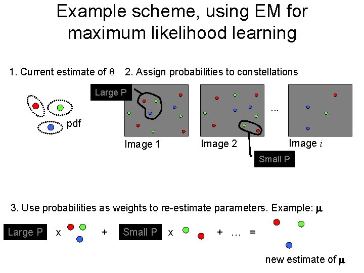
Example scheme, using EM for maximum likelihood learning 1. Current estimate of 2. Assign probabilities to constellations Large P . . . pdf Image 2 Image 1 Image i Small P 3. Use probabilities as weights to re-estimate parameters. Example: Large P x + Small P x + … = new estimate of

Learning Shape & Appearance simultaneously Fergus et al. ‘ 03